Lecture 8: Unsupervised Learning
Contents
Lecture 8: Unsupervised Learning#
Next, we shift our attention towards the second major class of machine learning algorithms: unsupervised learning.
8.1. Introduction to Unsupervised Learning#
In unsupervised learning, we start with a dataset that does not contain labels. Unsupervised learning seeks to discover interesting and useful patterns in this data, such as:
Clusters of related datapoints. For example, we might want to discover groups of similar customers from the logs of an e-commerce website.
Outliers, i.e., particularly unusual or interesting datapoints. For example, suspicious financial transactions.
Denoised signals. Recovering an image corrupted with white noise.
8.1.1. Unsupervised Learning: An Example#
To make things concrete, let’s look at an example of an unsupervised learning.
We can describe unsupervised learning via the following recipe, which is similar to the one we introduced in the context of supervised learning.
The unsupervised model is no longer a predictive model. Rather, it describes interesting structure in the data. For instance, it can identify clusters of related datapoints.
8.1.1.1. An Unsupervised Learning Dataset#
As an example of an unsupervised learning dataset, we will use the Iris flower data that we have previously seen in the context of supervised learning. To make things truly unsupervised, we will discard all the labels from this dataset.
Let’s start by loading this dataset.
# import standard machine learning libraries
import numpy as np
import pandas as pd
from sklearn import datasets

# Load the Iris dataset
iris = datasets.load_iris()

# Print out the description of the dataset
print(iris.DESCR)
.. _iris_dataset:

Iris plants dataset
--------------------

**Data Set Characteristics:**

    :Number of Instances: 150 (50 in each of three classes)
    :Number of Attributes: 4 numeric, predictive attributes and the class
    :Attribute Information:
        - sepal length in cm
        - sepal width in cm
        - petal length in cm
        - petal width in cm
        - class:
                - Iris-Setosa
                - Iris-Versicolour
                - Iris-Virginica

    :Summary Statistics:

    ============== ==== ==== ======= ===== ====================
                    Min  Max   Mean    SD   Class Correlation
    ============== ==== ==== ======= ===== ====================
    sepal length:   4.3  7.9   5.84   0.83    0.7826
    sepal width:    2.0  4.4   3.05   0.43   -0.4194
    petal length:   1.0  6.9   3.76   1.76    0.9490  (high!)
    petal width:    0.1  2.5   1.20   0.76    0.9565  (high!)
    ============== ==== ==== ======= ===== ====================

    :Missing Attribute Values: None
    :Class Distribution: 33.3% for each of 3 classes.
    :Creator: R.A. Fisher
    :Donor: Michael Marshall (MARSHALL%PLU@io.arc.nasa.gov)
    :Date: July, 1988

The famous Iris database, first used by Sir R.A. Fisher. The dataset is taken
from Fisher's paper. Note that it's the same as in R, but not as in the UCI
Machine Learning Repository, which has two wrong data points.

This is perhaps the best known database to be found in the
pattern recognition literature.  Fisher's paper is a classic in the field and
is referenced frequently to this day.  (See Duda & Hart, for example.)  The
data set contains 3 classes of 50 instances each, where each class refers to a
type of iris plant.  One class is linearly separable from the other 2; the
latter are NOT linearly separable from each other.

.. topic:: References

   - Fisher, R.A. "The use of multiple measurements in taxonomic problems"
     Annual Eugenics, 7, Part II, 179-188 (1936); also in "Contributions to
     Mathematical Statistics" (John Wiley, NY, 1950).
   - Duda, R.O., & Hart, P.E. (1973) Pattern Classification and Scene Analysis.
     (Q327.D83) John Wiley & Sons.  ISBN 0-471-22361-1.  See page 218.
   - Dasarathy, B.V. (1980) "Nosing Around the Neighborhood: A New System
     Structure and Classification Rule for Recognition in Partially Exposed
     Environments".  IEEE Transactions on Pattern Analysis and Machine
     Intelligence, Vol. PAMI-2, No. 1, 67-71.
   - Gates, G.W. (1972) "The Reduced Nearest Neighbor Rule".  IEEE Transactions
     on Information Theory, May 1972, 431-433.
   - See also: 1988 MLC Proceedings, 54-64.  Cheeseman et al"s AUTOCLASS II
     conceptual clustering system finds 3 classes in the data.
   - Many, many more ...
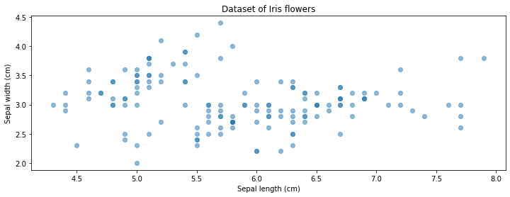
For simplicity, we will discard petal length and width and use only sepal length and width as the attributes of each datapoint. Importantly, we also discard the class label.
With each datapoint containing two attributes, we can visualize this dataset in 2D using the code below.
from matplotlib import pyplot as plt
plt.rcParams['figure.figsize'] = [12, 4]

# Visualize the Iris flower dataset
# iris.data[:,0] is the sepal length, while iris.data[:,1] is the sepal width
plt.scatter(iris.data[:,0], iris.data[:,1], alpha=0.5)
plt.ylabel("Sepal width (cm)")
plt.xlabel("Sepal length (cm)")
plt.title("Dataset of Iris flowers")
Fontconfig warning: ignoring UTF-8: not a valid region tag
Text(0.5, 1.0, 'Dataset of Iris flowers')
8.1.1.2. An Unsupervised Learning Algorithm#
We will use the above dataset as input to an important and popular unsupervised learning algorithm, \(K\)-means.
The algorithm seeks to find \(K\) clusters in the data.
Each cluster is characterized by its centroid (its mean).
The code below runs \(K\)-means, which is available in the sklearn libary, using \(K = 3\).
# fit K-Means with K=3
from sklearn import cluster
model = cluster.KMeans(n_clusters=3)
model.fit(iris.data[:,[0,1]])
KMeans(n_clusters=3)
The output of \(K\)-means are three cluster centroids: these are just three points in the space of \(x\). Let’s visualize them together with our dataset.
# visualize the datapoints
plt.scatter(iris.data[:,0], iris.data[:,1], alpha=0.5)
# visualize the learned clusters with red markers
plt.scatter(model.cluster_centers_[:,0], model.cluster_centers_[:,1], marker='D', c='r', s=100)
plt.ylabel("Sepal width (cm)")
plt.xlabel("Sepal length (cm)")
plt.title("Dataset of Iris flowers")
plt.legend(['Datapoints', 'Probability peaks'])
<matplotlib.legend.Legend at 0x7fa46a892130>
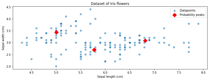
In the above figure, the red diamonds indicate the locations of the centroids.
It would be helpful to understand whether the centroids provided to us by \(K\)-means have been able to discover interesting structure in this unlabeled dataset. One way in which we could do this in this example is by leveraging the class labels, which we have originally discarded.
The figure below colors each datapoint according to its true class (which was not available to the \(K\)-means algorithm).
# visualize datapoints belonging to different classes with colors
p1 = plt.scatter(iris.data[:,0], iris.data[:,1], alpha=1, c=iris.target, cmap='Paired')
# visualize the learned cluster with red markers
plt.scatter(model.cluster_centers_[:,0], model.cluster_centers_[:,1], marker='D', c='r', s=100)
plt.ylabel("Sepal width (cm)")
plt.xlabel("Sepal length (cm)")
plt.title("Dataset of Iris flowers")
plt.legend(handles=p1.legend_elements()[0], labels=['Iris Setosa', 'Iris Versicolour', 'Iris Virginica'])
<matplotlib.legend.Legend at 0x7fa4990c40d0>
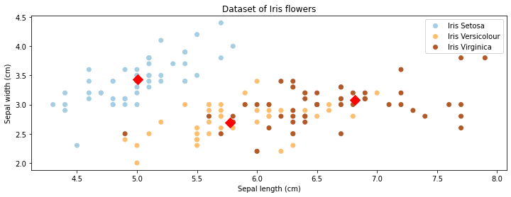
Interestingly, we find that the centroids approximately correspond to the three classes of flowers present in the dataset! The \(K\)-means algorithm was able to discover these without using any labels.
This example should help illustrate how interesting insights can be found using unsupervised learning from completely unlabeled data.
8.1.2. Applications of Unsupervised Learning#
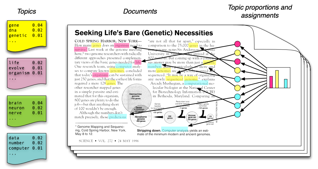
Unsupervised learning has many additional applications. One example that we introduced in the first lecture is topic modeling. Consider the following text, which contains at least four distinct topics. (image credit: David Blei)
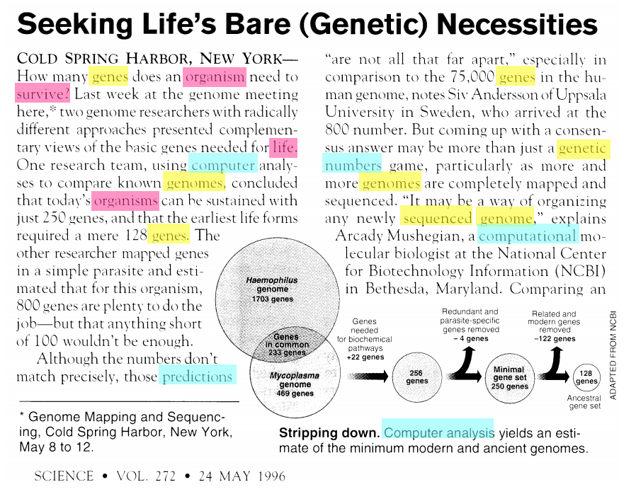
The blue words pertain mostly to computers. The red words pertain to biology. The yellow words are related to genetics.
It would be useful to be able to detect these topics automatically. However, in practice we rarely have access to text in which each word is labeled with a topic.
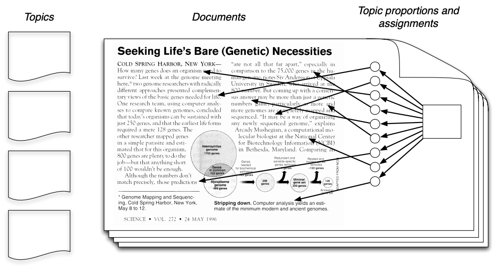
Unsupervised topic models automatically discover clusters of related words (these are the “topics”, e.g., computers) and assign a topic to each word, as well as a set of topic proportions to each document.
Other broad classes of use cases for unsupervised learning include:
Visualization: Projecting data into a lower-dimensional space in which it easier to identify and understanding interesting patterns.
Anomaly detection. The field of predictive maintenance seeks to identify factory components that are likely to fail soon.
Signal denoising. Extracting human speech from a noisy audio recording.
8.2. The Language of Unsupervised Learning#
Next, we will introduce notation and use it to identify the elements that define an unsupervised learning problem.
8.2.1. A Recipe for Unsupervised Learning#
At a high level, an unsupervised machine learning problem can be described by the following “recipe”, which is analogous to supervised learning.
To perform supervised learning, we first collect a dataset and define a learning algorithm. The result of running the algorithm on the data is an unsupervised learning model. The outputs of this model are interesting properties of the data.
More formally, we define an unsupervised dataset of size \(n\) as
Each \(x^{(i)} \in \mathbb{R}^d\) denotes an input, a vector of \(d\) attributes or features.
We can think of an unsupervised learning algorithm as consisting of three components:
A model class: the set of possible unsupervised models we consider.
An objective function, which defines how good a model is.
An optimizer, which finds the best predictive model in the model class according to the objective function
8.2.1.1. Model & Model Class#
We’ll say that a model is a function
that maps inputs \(x \in \mathcal{X}\) to some kind of structure \(s \in \mathcal{S}\). Models may have parameters \(\theta \in \Theta\) living in a set \(\Theta\) Structures can take many forms (clusters, low-dimensional representations, etc.), and we will see many examples.
Formally, the model class is a set
of possible models (models with different parameters) that map input features to structural elements.
8.2.1.3. Learning Objective#
We again define an objective function (also called a loss function)
which describes the extent to which \(f_\theta\) “fits” the data \(\mathcal{D} = \{x^{(i)} \mid i = 1,2,...,n\}\).
8.2.1.4. Optimizer#
An optimizer finds a model \(f_\theta \in \mathcal{M}\) with the smallest value of the objective \(J\).
Intuitively, this is the function that bests “fits” the data on the training dataset.
8.2.2. An Example: \(K\)-Means#
To better understand how these three components define an unsupervised learning algorithm, let’s derive the \(K\)-means algorithm that we have seen earlier in terms of these components.
Recall how we previously introduced the \(K\)-means algorithm:
The algorithm seeks to find \(K\) hidden clusters in the data.
Each cluster is characterized by its centroid (its mean).
8.2.2.1. K-Means: An Intuitive Explanation#
Before we define \(K\)-means formally, let’s define it somewhat more intuitively.
At a high level, \(K\)-means performs the following steps. Starting from random centroids, we repeat until convergence:
Update each cluster: assign each point to its closest centroid.
Set each centroid to be the center of the its cluster
This is best illustrated visually - see Wikipedia
In the above example, the big red “+”, yellow “-” and blue “\(\circ\)” symbols represent clusters. At each iteration, they get recomputed to the center of the red, yellow, and blue points respectively. After they are recomputed, the datapoints are re-colored to match the color of their closest centroid.
8.2.2.2. The \(K\)-Means Model#
More formally, the parameters \(\theta\) of the model are \(K\) centroids \(c_1, c_2, \ldots c_K \in \mathcal{X}\). The class of \(x\) is going to be \(k\) if \(c_k\) is the closest centroid to \(x\) (for this lecture, let’s assume the distance metric in use is Euclidean distance, although the algorithm works with any distance metric).
We can think of the model returned by \(K\)-Means as a function
that assigns each input \(x\) to a cluster \(s \in \mathcal{S} = \{1,2,\ldots,K\}\).
8.2.2.3. The \(K\)-Means Objective#
How do we determine whether \(f_\theta\) is a good clustering of the dataset \(\mathcal{D}\)?
We seek centroids \(c_k\) such that the distance between the points and their closest centroid is minimized:
where \(\text{centroid}(k) = c_k\) denotes the centroid for cluster \(k\).
8.2.2.4. The \(K\)-Means Optimizer#
We can optimize this in a two-step process, starting with an initial random cluster assignment \(f_\theta(x)\).
Starting with random centroids \(c_k\), repeat until convergence:
Update \(f(x)\) such that \(f(x^{(i)}) = \arg\min_k ||x^{(i)} - c_k||\) is the cluster of the closest centroid to \(x^{(i)}\).
Set each \(c_k\) to be the center of its cluster \(\{x^{(i)} \mid f(x^{(i)}) = k\}\).
Though we do not prove it here, this process is guaranteed to converge after a finite number of iterations. The intuition is that the objective function decreases at each step, hence at some point it must reach an optimum
8.2.2.5. Algorithm: K-Means#
This completes our definition of \(K\)-means in terms of its model, objective, and optimizer. This definition is now sufficiently precise for you to implement this algorithm from scratch. In fact, in the next lecture, we will implement an improved version of this algorithm.
As with previous supervised algorithms, we provide a model card for \(K\)-means in terms of its standard components:
Type: Unsupervised learning (clustering)
Model family: \(k\) centroids
Objective function: Sum of distances (of your choice) to the closest centroids
Optimizer: Iterative optimization procedure.
8.3. Unsupervised Learning in Practice#
We conclude this lecture with some practical considerations to keep in mind when applying unsupervised learning.
Recall that in supervised learning, generalization is the property of predictive models to achieve good performance on new, holdout data that is distinct from the training set.
How does generalization apply to unsupervised learning?
8.3.0. An Unsupervised Learning Dataset#
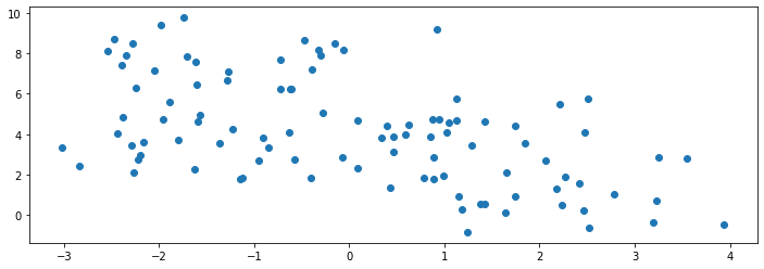
As a running example for this subsection, consider the following dataset, consisting of datapoints generated by a mixture of four Gaussian distributions. A sample from this mixture distribution should form roughly four clusters.
We visualize a sample of 100 datapoints below:
# import libraries
import numpy as np
from sklearn import datasets
from matplotlib import pyplot as plt
plt.rcParams['figure.figsize'] = [12, 4]

# Setting the seed makes the random module of numpy deterministic across different runs of the program
np.random.seed(0)
# Generate random 2D datapoints using 4 different Gaussians.
X, y = datasets.make_blobs(centers=4)
plt.scatter(X[:,0], X[:,1])
<matplotlib.collections.PathCollection at 0x7fa488a7a700>
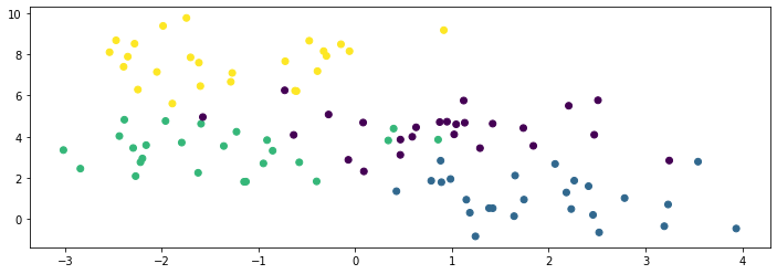
We know the true labels of these clusters, i.e., which Gaussian a datapoint is generated by, so we can visualize them with different colors below:
plt.scatter(X[:,0], X[:,1], c=y)
<matplotlib.collections.PathCollection at 0x7fa46ab33df0>
8.3.1. Underfitting in Unsupervised Learning#
In supervised learning, underfitting occurs when our model is too simple to fit the data.
Similarly, in unsupervised learning, underfitting happens when we are not able to fully learn the signal present in the data. In the context of \(K\)-Means, this means our \(K\) is lower than the actual number of clusters in the data.
Let’s run \(K\)-Means on our toy dataset.
# fit a K-Means
from sklearn import cluster
model = cluster.KMeans(n_clusters=2)
model.fit(X)
KMeans(n_clusters=2)
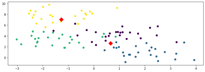
The centroids find two distinct components (or clusters) in the data, but they fail to capture the true structure.
Below, we visualize both the datapoints and the learned clusters. You can see that more than one true cluster (represented by different colors) is associated to a learned cluster.
plt.scatter(X[:,0], X[:,1], c=y)
plt.scatter(model.cluster_centers_[:,0], model.cluster_centers_[:,1], marker='D', c='r', s=100)
print('K-Means Objective: %.2f' % -model.score(X))
K-Means Objective: 462.03
8.3.4. Overfitting in Unsupervised Learning#
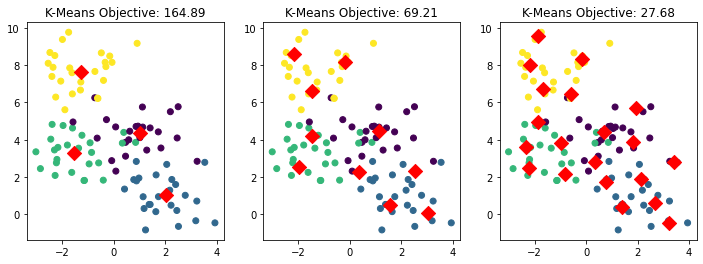
Overfitting happens when we fit the noise, but not the signal. In our example, this means fitting small, local noise clusters rather than the true global clusters.
Consider what happens if we further increase \(K\) in our earlier example. In the figures below, we set \(K\) equal to 4, 10, and 20 from left to right respectively.
# Will visualize learned clusters of K-means with different Ks.
Ks = [4, 10, 20]
f, axes = plt.subplots(1,3)
for k, ax in zip(Ks, axes):
    # Fit K-means
    model = cluster.KMeans(n_clusters=k)
    model.fit(X)
    # Visual both the datapoints and the k learned clusters
    ax.scatter(X[:,0], X[:,1], c=y)
    ax.scatter(model.cluster_centers_[:,0], model.cluster_centers_[:,1], marker='D', c='r', s=100)
    ax.set_title('K-Means Objective: %.2f' % -model.score(X))
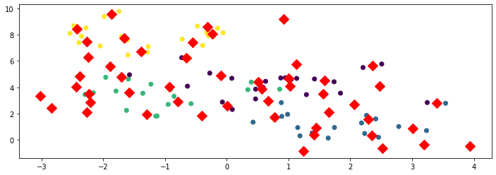
We can take this one step further by setting \(K = 50\) below.
# Setting K = 50
model = cluster.KMeans(n_clusters=50)
# Fit K-means
model.fit(X)
# Visualize both the datapoints and the learned clusters
plt.scatter(X[:,0], X[:,1], c=y)
plt.scatter(model.cluster_centers_[:,0], model.cluster_centers_[:,1], marker='D', c='r', s=100)
print('K-Means Objective: %.2f' % -model.score(X))
K-Means Objective: 4.67
8.3.5. Generalization in Unsupervised Learning#
To talk about generalization, we usually assume that the dataset is sampled from a probability distribution \(\mathbb{P}\), which we will call the data distribution. We will denote this as
Moreover, we assume the dataset \(\mathcal{D} = \{x^{(i)} \mid i = 1,2,...,n\}\) consists of independent and identically distributed (IID) samples from \(\mathbb{P}\).
What independent and identically distributed (IID) means is:
Each training example is from the same distribution.
This distribution doesn’t depend on previous training examples.
Example: Flipping a coin. Each flip has the same probability of heads & tails and doesn’t depend on previous flips.
Counter-Example: Yearly census data. The population in each year will be close to that of the previous year.
We can think of the data distribution as being the sum of two distinct components \(\mathbb{P} = F + E\)
A signal component \(F\) (hidden clusters, speech, low-dimensional data space, etc.)
A random noise component \(E\)
A machine learning model generalizes if it fits the true signal \(F\); it overfits if it learns the noise \(E\). This definition is less precise than the one we introduced initially in the context of supervised learning; however, it is also more general and applies to unsupervised learning algorithms.
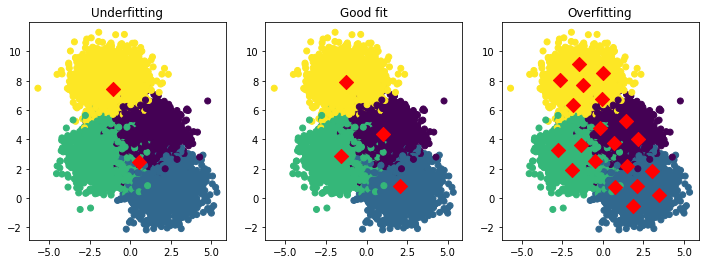
Below, we visualize examples of underfitting, a good fit, and overfitting in the context of our running example with \(K\)-means.
Ks, titles = [2, 4, 20], ['Underfitting', 'Good fit', 'Overfitting']
f, axes = plt.subplots(1,3)
for k, title, ax in zip(Ks, titles, axes):
    model = cluster.KMeans(n_clusters=k)
    model.fit(X)
    ax.scatter(X[:,0], X[:,1], c=y)
    ax.scatter(model.cluster_centers_[:,0], model.cluster_centers_[:,1], marker='D', c='r', s=100)
    ax.set_title(title)
8.3.5.1. Detecting Overfitting and Underfitting#
In real-life scenarios when our data is not two-dimensional, visualizing the data and the cluster centers might not help us detect overfitting or underfitting. We would also not have access to the true cluster labels.
Generally, in unsupervised learning, overfitting and underfitting are more difficult to quantify than in supervised learning because:
Performance may depend on our intuition and require human evaluation
If we know the true labels, we can measure the accuracy of the clustering. But we do not have labels for unsupervised learning.
If our model is probabilistic, one thing that we can do to detect overfitting without labels is to compare the log-likelihood between the training set and a holdout set (see the next lecture).
8.3.5.2. The Elbow Method#
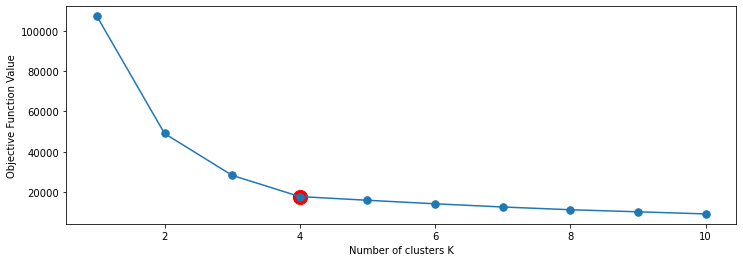
The elbow method is a useful heuristic that can be used to tune hyper-parameters in unsupervised learning, e.g., choosing \(K\) for \(K\)-means. The elbow method works as follows:
We plot the objective function as a function of the hyper-parameter \(K\).
The “elbow” of the curve happens when its rate of decrease substantially slows down.
The “elbow’ is a good guess for the hyperparameter.
In our example, the decrease in objective values slows down after \(K=4\), and after that, the curve becomes just a line. Below we plot the graph of objective function value vs \(K\). You can see that at \(K = 4\), our objective value does not improve too much anymore even if we increase \(K\).
Ks, objs = range(1,11), []
for k in Ks:
    model = cluster.KMeans(n_clusters=k)
    model.fit(X)
    objs.append(-model.score(X))

plt.plot(Ks, objs, '.-', markersize=15)
plt.scatter([4], [objs[3]], s=200, c='r')
plt.xlabel("Number of clusters K")
plt.ylabel("Objective Function Value")
Text(0, 0.5, 'Objective Function Value')
8.3.5.3. Reducing Overfitting#
Choosing hyper-parameters via the elbow method is one thing you can do to avoid overfitting. In general, there are multiple ways to control overfitting including:
Reduce model complexity (e.g., reduce \(K\) in \(K\)-Means)
Penalize complexity in the objective (e.g., penalize large \(K\))
Use a probabilistic model and regularize it.
8.3.5.4. Generalization in Unsupervised Learning: Summary#
As you can see, the concept of generalization applies to both supervised and unsupervised learning.
In supervised learning, it is easier to quantify via accuracy.
In unsupervised learning, we may not be able to easily detect overfitting, but it still happens. We have discussed practical methods to diagnose and reduce overfitting.