Lecture 13: Dual Formulation of Support Vector Machines
Contents
Lecture 13: Dual Formulation of Support Vector Machines#
In this lecture, we will see a different formulation of the SVM called the dual. This dual formulation will lead to new types of optimization algorithms with favorable computational properties in scenarios when the number of features is very large (and possibly even infinite!).
13.1. Lagrange Duality#
Before we define the dual of the SVM problem, we need to introduce some additional concepts from optimization, namely Lagrange duality.
13.1.1. Review: Classification Margins#
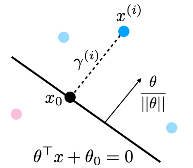
In the previous lecture, we defined the concept of classification margins. Recall that the margin \(\gamma^{(i)}\) is the distance between the separating hyperplane and the datapoint \(x^{(i)}\).
Large margins are good, since data should be far from the decision boundary. Maximizing the margin of a linear model amounts to solving the following optimization problem:
We are now going to look at a different way of optimizing this objective. But first, we need to define Lagrange duality.
13.1.2. Lagrange Duality in Constrained Optimization#
We start by introducing the definition of a constrained optimization problem. We will look at constrained optimization problems of the form
where \(J(\theta)\) is the optimization objective and each \(c_k(\theta) : \mathbb{R}^d \to \mathbb{R}\) is a constraint.
Our goal is to find a small value of \(J(\theta)\) such that the \(c_k(\theta)\) are negative. Rather than solving the above problem, we can solve the following related optimization problem, which contains additional penalty terms:
This new objective includes an additional vector of Lagrange multipliers \(\lambda \in [0, \infty)^K\), which are positive weights that we place on the constraint terms. We call \(\mathcal{L}(\theta, \lambda)\) the Lagrangian. Observe that:
If \(\lambda_k \geq 0\), then we penalize large values of \(c_k\)
For large enough \(\lambda_k\), no \(c_k\) will be positive—a valid solution.
Thus, penalties are another way of enforcing constraints.
13.1.2.1. The Primal Lagrange Form#
Consider again our constrained optimization problem:
We define its primal Lagrange form to be
These two forms have the same optimum \(\theta^*\)! The reason for this to be true can be proved considering the following:
Observe that:
If a \(c_k\) is violated (\(c_k > 0\)) then \(\max_{\lambda \geq 0} \mathcal{L}(\theta, \lambda)\) is \(\infty\) as \(\lambda_k \to \infty\).
If no \(c_k\) is violated and \(c_k < 0\) then the optimal \(\lambda_k = 0\) (any bigger value makes the inner objective smaller).
If \(c_k < 0\) for all \(k\) then \(\lambda_k=0\) for all \(k\) and $\( \min_{\theta \in \mathbb{R}^d} \mathcal{P}(\theta) = \min_{\theta \in \mathbb{R}^d} \max_{\lambda \geq 0} \mathcal{L}(\theta, \lambda) = \min_{\theta \in \mathbb{R}^d} J(\theta) \)$
Thus, \(\min_{\theta \in \mathbb{R}^d} \mathcal{P}(\theta)\) is the solution to our original optimization problem.
13.1.2.2. The Dual Lagrange Form#
Now consider the following problem over \(\lambda\geq 0\): $\( \max_{\lambda \geq 0}\mathcal{D}(\lambda) = \max_{\lambda \geq 0} \min_{\theta \in \mathbb{R}^d} \mathcal{L}(\theta, \lambda) = \max_{\lambda \geq 0} \min_{\theta \in \mathbb{R}^d} \left(J(\theta) + \sum_{k=1}^K \lambda_k c_k(\theta) \right). \)$
We call this the Lagrange dual of the primal optimization problem \(\min_{\theta \in \mathbb{R}^d} \mathcal{P}(\theta)\). We can always construct a dual for the primal.
13.1.2.3. Lagrange Duality#
Once we have constructed a dual for the primal, the dual would be interesting because we always have: $\( \max_{\lambda \geq 0}\mathcal{D}(\lambda) = \max_{\lambda \geq 0} \min_{\theta \in \mathbb{R}^d} \mathcal{L}(\theta, \lambda) \leq \min_{\theta \in \mathbb{R}^d} \max_{\lambda \geq 0} \mathcal{L}(\theta, \lambda) = \min_{\theta \in \mathbb{R}^d} \mathcal{P}(\theta)\)$
Moreover, in many cases, we have $\( \max_{\lambda \geq 0}\mathcal{D}(\lambda) = \min_{\theta \in \mathbb{R}^d} \mathcal{P}(\theta). \)$ Thus, the primal and the dual are equivalent! This is very important and we will use this feature for moving into the next steps of solving SVMs.
13.1.3. An Aside: Constrained Regularization#
Before we move on to defining the dual form of SVMs, we want to make a brief side comment on the related topic of constrained regularization. Consider a regularized supervised learning problem with a penalty term: $\( \min_{\theta \in \Theta} L(\theta) + \gamma \cdot R(\theta). \)$
We may also enforce an explicit constraint on the complexity of the model:
We will not prove this, but solving this problem is equivalent so solving the penalized problem for some \(\gamma > 0\) that’s different from \(\gamma'\). In other words, we can regularize by explicitly enforcing \(R(\theta)\) to be less than a value or we can penalize \(R(\theta)\).
13.2. Dual Formulation of SVMs#
Let’s now apply Lagrange duality to support vector machines.
13.2.1. Review: Max-Margin Classification#
First, let’s briefly reintroduce the task of binary classification using a linear model and a max-margin objective.
Consider a training dataset \(\mathcal{D} = \{(x^{(1)}, y^{(1)}), (x^{(2)}, y^{(2)}), \ldots, (x^{(n)}, y^{(n)})\}\). We distinguish between two types of supervised learning problems depending on the targets \(y^{(i)}\).
Regression: The target variable \(y \in \mathcal{Y}\) is continuous: \(\mathcal{Y} \subseteq \mathbb{R}\).
Binary Classification: The target variable \(y\) is discrete and takes on one of \(K=2\) possible values.
In this lecture, we assume \(\mathcal{Y} = \{-1, +1\}\). We will also work with linear models of the form:
where \(x \in \mathbb{R}^d\) is a vector of features and \(y \in \{-1, 1\}\) is the target. The \(\theta_j\) are the parameters of the model.
We can represent the model in a vectorized form
We define the geometric margin \(\gamma^{(i)}\) with respect to a training example \((x^{(i)}, y^{(i)})\) as $\( \gamma^{(i)} = y^{(i)}\left( \frac{\theta^\top x^{(i)} + \theta_0}{||\theta||} \right). \)\( This also corresponds to the distance from \)x^{(i)}$ to the hyperplane.
We saw that maximizing the margin of a linear model amounts to solving the following optimization problem.
13.2.2. The Dual of the SVM Problem#
Let’s now derive the SVM dual. Consider the following objective, the Lagrangian of the max-margin optimization problem.
We have put each constraint inside the objective function and added a penalty \(\lambda_i\) to it.
Recall that the following formula is the Lagrange dual of the primal optimization problem \(\min_{\theta \in \mathbb{R}^d} \mathcal{P}(\theta)\). We can always construct a dual for the primal. $\(\max_{\lambda \geq 0}\mathcal{D}(\lambda) = \max_{\lambda \geq 0} \min_{\theta \in \mathbb{R}^d} \mathcal{L}(\theta, \lambda) = \max_{\lambda \geq 0} \min_{\theta \in \mathbb{R}^d} \left(J(\theta) + \sum_{k=1}^K \lambda_k c_k(\theta) \right).\)$
It is easy to write out the dual form of the max-margin problem. Consider optimizing the above Lagrangian over \(\theta, \theta_0\) for any value of \(\lambda\).
This objective is quadratic in \(\theta\); hence it has a single minimum in \(\theta\).
We can find it by setting the derivative to zero and solving for \(\theta, \theta_0\):
Substituting this into the Lagrangian we obtain the following expression for the dual \(\max_{\lambda\geq 0} \mathcal{D}(\lambda) = \max_{\lambda\geq 0} \min_{\theta, \theta_0} L(\theta, \theta_0, \lambda)\):
13.2.3. Properties of SVM Duals#
Recall that in general, we have:
In the case of the SVM problem, one can show that
Thus, the primal and the dual are equivalent!
We can also make several other observations about this dual:
This is a constrained quadratic optimization problem.
The number of variables \(\lambda_i\) equals \(n\), the number of data points.
Objective only depends on products \((x^{(i)})^\top x^{(j)}\) (keep reading for more on this!)
13.2.3.1. When to Solve the Dual#
An interesting question arises when we need to decide which optimization problem to solve: the dual or the primal. In short, the deciding factor is the number of features (the dimensionality of \(x\)) relative to the number of datapoints:
The dimensionality of the primal depends on the number of features. If we have a few features and many datapoints, we should use the primal.
Conversely, if we have a lot of features, but fewer datapoints, we want to use the dual.
In the next lecture, we will see how we can use this property to solve machine learning problems with a very large number of features (even possibly infinite!).
13.3. Practical Considerations for SVM Duals#
In this part, we will continue our discussion of the dual formulation of the SVM with additional practical details.
Recall that the the max-margin hyperplane can be formulated as the solution to the following primal optimization problem.
The solution to this problem also happens to be given by the following dual problem:
13.3.1. Non-Separable Problems#
Our dual problem assumes that a separating hyperplane exists. If it doesn’t, our optimization problem does not have a solution, and we need to modify it. Our approach is going to be to make each constraint “soft”, by introducing “slack” variables, which allow the constraint to be violated.
In the optimization problem, we assign a penalty \(C\) to these slack variables to obtain:
This is the primal problem. Let’s now form its dual. First, the Lagrangian \(L(\lambda, \mu,\theta,\theta_0,\xi)\) equals
The dual objective of this problem will equal
As earlier, we can solve for the optimal \(\theta, \theta_0\) in closed form and plug back the resulting values into the objective. We can then show that the dual takes the following form:
13.3.2. Sequential Minimal Optimization and Coordinate Descent#
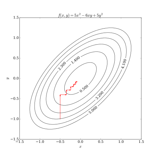
Coordinate descent is a general way to optimize functions \(f(x)\) of multiple variables \(x \in \mathbb{R}^d\). It executes as:
Choose a dimension \(j \in \{1,2,\ldots,d\}\).
Optimize \(f(x_1, x_2, \ldots, x_j, \ldots, x_d)\) over \(x_j\) while keeping the other variables fixed.
Here, we visualize coordinate descent applied to a 2D quadratic function.
We can apply a form of coordinate descent to solve the dual:
A popular, efficient algorithm is Sequential Minimal Optimization (SMO), which executes as:
Take a pair \(\lambda_i, \lambda_j\), possibly using heuristics to guide choice of \(i,j\).
Reoptimize over \(\lambda_i, \lambda_j\) while keeping the other variables fixed.
Repeat the above until convergence.
13.3.3. Obtaining a Primal Solution from the Dual#
Next, assuming we can solve the dual, how do we find a separating hyperplane \(\theta, \theta_0\)?
Recall that we already found an expression for the optimal \(\theta^*\) (in the separable case) as a function of \(\lambda\):
Once we know \(\theta^*\) it easy to check that the solution to \(\theta_0\) is given by
13.3.4. Support Vectors#
A powerful property of the SVM dual is that at the optimum, most variables \(\lambda_i\) are zero! Thus, \(\theta\) is a sum of a small number of points:
The points for which \(\lambda_i > 0\) are precisely the points that lie on the margin (are closest to the hyperplane).
These are called support vectors, and this is where the SVM algorithm takes its name. We are going to illustrate the concept of an SVM using a figure.
13.3.5. A Hands-On Example#
Let’s look at a concrete example of how to use the dual version of the SVM. In this example, we are going to again use the Iris flower dataset. We will merge two of the three classes to make it suitable for binary classification.
import numpy as np
import pandas as pd
from sklearn import datasets

# Load the Iris dataset
iris = datasets.load_iris(as_frame=True)
iris_X, iris_y = iris.data, iris.target

# subsample to a third of the data points
iris_X = iris_X.loc[::4]
iris_y = iris_y.loc[::4]

# create a binary classification dataset with labels +/- 1
iris_y2 = iris_y.copy()
iris_y2[iris_y2==2] = 1
iris_y2[iris_y2==0] = -1

# print part of the dataset
pd.concat([iris_X, iris_y2], axis=1).head()
| sepal length (cm) | sepal width (cm) | petal length (cm) | petal width (cm) | target | |
|---|---|---|---|---|---|
| 0 | 5.1 | 3.5 | 1.4 | 0.2 | -1 |
| 4 | 5.0 | 3.6 | 1.4 | 0.2 | -1 |
| 8 | 4.4 | 2.9 | 1.4 | 0.2 | -1 |
| 12 | 4.8 | 3.0 | 1.4 | 0.1 | -1 |
| 16 | 5.4 | 3.9 | 1.3 | 0.4 | -1 |
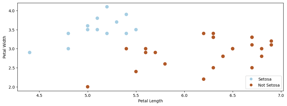
Let’s visualize this dataset.
# https://scikit-learn.org/stable/auto_examples/neighbors/plot_classification.html
%matplotlib inline
import matplotlib.pyplot as plt
plt.rcParams['figure.figsize'] = [12, 4]
import warnings
warnings.filterwarnings("ignore")

# create 2d version of dataset and subsample it
X = iris_X.to_numpy()[:,:2]
x_min, x_max = X[:, 0].min() - .5, X[:, 0].max() + .5
y_min, y_max = X[:, 1].min() - .5, X[:, 1].max() + .5
xx, yy = np.meshgrid(np.arange(x_min, x_max, .02), np.arange(y_min, y_max, .02))

# Plot also the training points
p1 = plt.scatter(X[:, 0], X[:, 1], c=iris_y2, s=60, cmap=plt.cm.Paired)
plt.xlabel('Petal Length')
plt.ylabel('Petal Width')
plt.legend(handles=p1.legend_elements()[0], labels=['Setosa', 'Not Setosa'], loc='lower right')
<matplotlib.legend.Legend at 0x7f8311ce5550>
We can run the dual version of the SVM by importing an implementation from sklearn:
#https://scikit-learn.org/stable/auto_examples/svm/plot_separating_hyperplane.html
from sklearn import svm

# fit the model, don't regularize for illustration purposes
clf = svm.SVC(kernel='linear', C=1000) # this optimizes the dual
# clf = svm.LinearSVC() # this optimizes for the primal
clf.fit(X, iris_y2)

plt.scatter(X[:, 0], X[:, 1], c=iris_y2, s=30, cmap=plt.cm.Paired)
Z = clf.decision_function(np.c_[xx.ravel(), yy.ravel()]).reshape(xx.shape)

# plot decision boundary and margins
plt.contour(xx, yy, Z, colors='k', levels=[-1, 0, 1], alpha=0.5,
           linestyles=['--', '-', '--'])
plt.scatter(clf.support_vectors_[:, 0], clf.support_vectors_[:, 1], s=100,
           linewidth=1, facecolors='none', edgecolors='k')
plt.xlim([4.6, 6])
plt.ylim([2.25, 4])
plt.show()
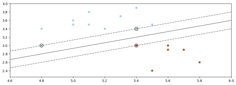
We can see that the solid line defines the decision boundary, and the two dotted lines are the geometric margin.
The data points that fall on the margin are the support vectors. Notice that only these vectors determine the position of the hyperplane. If we “wiggle” any of the other points, the margin remains unchanged—therefore the max-margin hyperplane also remains unchanged. However, moving the support vectors changes both the optimal margin and the optimal hyperplane.
This observation provides an intuitive explanation for the formula
In this formula, \(\lambda_i > 0\) only for the \(x^{(i)}\) that are support vectors. Hence, only these \(x^{(i)}\) influence the position of the hyperplane, which matches our earlier intuition.
13.3.6. Algorithm: Support Vector Machine Classification (Dual Form)#
In summary, the SVM algorithm can be succinctly defined by the following key components.
Type: Supervised learning (binary classification)
Model family: Linear decision boundaries.
Objective function: Dual of SVM optimization problem.
Optimizer: Sequential minimal optimization.
Probabilistic interpretation: No simple interpretation!
In the next lecture, we will combine dual SVMs with a new idea called kernels, which enable them to handle a very large number of features (and even an infinite number of features) without any additional computational cost.