Lecture 10: Clustering
Contents
Lecture 10: Clustering#
This lecture looks at a new unsupervised learning task: clustering.
10.1. Gaussian Mixture Models for Clustering#
We start by defining the clustering task and outlining some clustering algorithms.
10.1.1. Review: Unsupervised Learning#
We have a dataset without labels. Our goal is to learn something interesting about the structure of the data. Two related problems in the area of unsupervised learning we have looked at are clustering and density estimation
Clustering is the problem of identifying distinct components in the data. Usually, we apply clustering when we assume that the data will have a certain structure, specifically:
Datapoints in a cluster are more similar to each other than to points in other clusters
Clusters are usually defined by their centers, and potentially by other shape parameters.
A simple clustering algorithm we have looked at is \(K\)-Means
Density Estimation is the problem of learning a probabilistic model \(P_\theta(x) : \mathcal{X} \to [0,1]\) on an unsupervised dataset \(\mathcal{D}\) to approximate the true data distribution \(P_\text{data}\).
If we successfully learn \(P_\theta \approx P_\text{data}\), then we can use \(P_\theta\) to solve many downstream tasks, including generation, outlier detection, and also clustering.
In this lecture, we will introduce Gaussian mixture models as a type of probabilistic model \(P_\theta(x)\), as well as the expectation maximization algorithm to learn these models. This approach will involve both density estimation and clustering.
10.1.2. Gaussian Mixture Models (GMM)#
Gaussian mixtures is a probabilistic model of the form:
\(z \in \mathcal{Z} = \{1,2,\ldots,K\}\) is discrete and follows a categorical distribution \(P_\theta(z=k) = \phi_k\).
\(x \in \mathbb{R}\) is continuous; conditioned on \(z=k\), it follows a Normal distribution \(P_\theta(x | z=k) = \mathcal{N}(\mu_k, \Sigma_k)\).
The parameters \(\theta\) are the \(\mu_k, \Sigma_k, \phi_k\) for all \(k=1,2,\ldots,K\).
The model postulates that:
Our observed data is comprised of \(K\) clusters with proportions specified by \(\phi_1,\phi_2, \ldots, \phi_K\)
The points within each cluster follow a Normal distribution \(P_\theta(x | z=k) = \mathcal{N}(\mu_k, \Sigma_k)\).
Within this setup, \(z^{(i)}\) can be thought of as the cluster label for the data point \(x^{(i)}\); it can be obtained from \(P(z|x^{(i)})\)
A GMM also specifies a formula for the distribution \(P_\theta (x)\); we simply need to sum over the joint distribution as follows:
10.1.3. Clustering With Known Cluster Assignments#
Let’s first think about how we would do clustering if the identity of each cluster is known.
Specifically, let our dataset be \(\mathcal{D} = \{(x^{(1)}, z^{(1)}), (x^{(2)}, z^{(2)}), \ldots, (x^{(n)}, z^{(n)})\}\)
\(x^{(i)} \in \mathbb{R}\) are the datapoints we cluster
\(z^{(i)} \in \{1,2,...,K\}\) are the cluster IDs
We want to fit a GMM, where \(\mu_k\) represent the cluster centroids.
This is the same problem as in Gaussian Discriminant Analysis (GDA). We can fit a GMM to this data as follows:
We fit the parameters \(\phi_k\) to be % of each class \(k\) in \(\mathcal{D}\).
We fit the parameters \(\mu_k, \Sigma_k\) to be means and variances of each class \(k\).
We can infer the cluster ID \(z\) of new points using \(P(z|x)\) as in GDA.
Let’s look at an example on our Iris flower dataset. Below, we load the dataset:
import numpy as np
import pandas as pd
import warnings
warnings.filterwarnings('ignore')
from sklearn import datasets

# Load the Iris dataset
iris = datasets.load_iris(as_frame=True)

# print part of the dataset
iris_X, iris_y = iris.data, iris.target
pd.concat([iris_X, iris_y], axis=1).head()
| sepal length (cm) | sepal width (cm) | petal length (cm) | petal width (cm) | target | |
|---|---|---|---|---|---|
| 0 | 5.1 | 3.5 | 1.4 | 0.2 | 0 |
| 1 | 4.9 | 3.0 | 1.4 | 0.2 | 0 |
| 2 | 4.7 | 3.2 | 1.3 | 0.2 | 0 |
| 3 | 4.6 | 3.1 | 1.5 | 0.2 | 0 |
| 4 | 5.0 | 3.6 | 1.4 | 0.2 | 0 |
Recall that we have previously seen how to fit GMMs on a labeled \((x,y)\) dataset using maximum likelihood.
Let’s try this on our Iris dataset again (recall that this is called GDA). Below, we estimate/fit the parameters of the GMM.
# we can implement these formulas over the Iris dataset
X = iris_X.to_numpy()[:,:2]
d = 2 # number of features in our toy dataset
K = 3 # number of classes
n = X.shape[0] # size of the dataset

# these are the shapes of the parameters
mus = np.zeros([K,d])
Sigmas = np.zeros([K,d,d])
phis = np.zeros([K])

# we now compute the parameters
for k in range(3):
    X_k = X[iris_y == k]
    mus[k] = np.mean(X_k, axis=0)
    Sigmas[k] = np.cov(X_k.T)
    phis[k] = X_k.shape[0] / float(n)
The code below generates predictions from the GMM model that we just learned by implementing Bayes’ rule:
# we can implement this in numpy
def gda_predictions(x, mus, Sigmas, phis):
    """This returns class assignments and p(y|x) under the GDA model.

    We compute \arg\max_y p(y|x) as \arg\max_y p(x|y)p(y)
    """
    # adjust shapes
    n, d = x.shape
    x = np.reshape(x, (1, n, d, 1))
    mus = np.reshape(mus, (K, 1, d, 1))
    Sigmas = np.reshape(Sigmas, (K, 1, d, d))

    # compute probabilities
    py = np.tile(phis.reshape((K,1)), (1,n)).reshape([K,n,1,1])
    pxy = (
        np.sqrt(np.abs((2*np.pi)**d*np.linalg.det(Sigmas))).reshape((K,1,1,1))
        * -.5*np.exp(
            np.matmul(np.matmul((x-mus).transpose([0,1,3,2]), np.linalg.inv(Sigmas)), x-mus)
        )
    )
    pyx = pxy * py
    return pyx.argmax(axis=0).flatten(), pyx.reshape([K,n])

idx, pyx = gda_predictions(X, mus, Sigmas, phis)
We can visualize the GMM as follows:
# https://scikit-learn.org/stable/auto_examples/neighbors/plot_classification.html
%matplotlib inline
from matplotlib import pyplot as plt
from matplotlib.colors import LogNorm
plt.rcParams['figure.figsize'] = [12, 4]

x_min, x_max = X[:, 0].min() - .5, X[:, 0].max() + .5
y_min, y_max = X[:, 1].min() - .5, X[:, 1].max() + .5
xx, yy = np.meshgrid(np.arange(x_min, x_max, .02), np.arange(y_min, y_max, .02))
Z, pyx = gda_predictions(np.c_[xx.ravel(), yy.ravel()], mus, Sigmas, phis)
logpy = np.log(-1./3*pyx)

# Put the result into a color plot
Z = Z.reshape(xx.shape)
contours = np.zeros([K, xx.shape[0], xx.shape[1]])
for k in range(K):
    contours[k] = logpy[k].reshape(xx.shape)
for k in range(K):
    plt.contour(xx, yy, contours[k], levels=np.logspace(0, 1, 1))

# Plot also the training points
plt.scatter(X[:, 0], X[:, 1], c=iris_y, edgecolors='k', cmap=plt.cm.Paired)
plt.xlabel('Sepal length')
plt.ylabel('Sepal width')

plt.show()
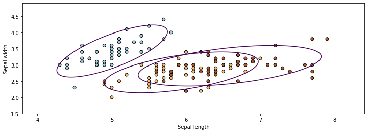
In the figure above, the ellipses represent the Gaussians, while the dots with different colors are the datapoints belonging to different classes. The \(P_\theta(z|x)\) from the GMM \(P_\theta\) can be used to obtain the cluster ID \(z\) of \(x\) (in fact, \(P_\theta(z|x)\) provides soft cluster assignments in the form of a probability distribution over \(z\)).
In this example, we straightforwardly trained the GMM \(P_\theta\) by maximizing likelihood since we know the label of each datapoint, i.e., which cluster it belongs to. But what if we don’t have labels to train \(P_\theta\)?
10.1.4. From Labeled to Unlabeled Clustering#
We will now see how to train a GMM clustering model from unlabeled data.
Our strategy will be to jointly learn cluster parameters and labels:
We will define an objective that does not require cluster labels \(z^{(i)}\).
We will define an optimizer that jointly infers both labels \(z^{(i)}\) and cluster parameters \(\mu_k, \Sigma_k\).
10.1.4.1. Maximum Marginal Likelihood Learning#
Maximum marginal (log-)likelihood is a way of learning a probabilistic model on an unsupervised dataset \(\mathcal{D}\) by maximizing:
This asks \(P_\theta\) to assign a high probability to the unlabeled training data \(x\) in \(\mathcal{D}\).
However, we need to use \(P(x) = \sum_{z \in \mathcal{Z}} P(x,z)\) to compute this probability because \(z\) is not observed.
Since our objective is
Note that by maximizing marginal likelihood we are asking the model to assign high probability to the data, just like in regular likelihood maximization. This also means that we are asking \(\sum_{z \in \mathcal{Z}} P_\theta({x}^{(i)}, z)\) to be high for at least one z.
Recall that the Kullback-Leibler (KL) divergence \(D(\cdot\|\cdot)\) between the model distribution and the data distribution is:
Note that maximizing the marginal likelihood is also equivalent to minimizing the KL divergence between the data and the model distribution.
The main disadvantage of marginal likelihood estimation is that this objective is much more difficult to optimize than previously. The learning objective will have multiple local optima and even computing its value at one \(\theta\) may be hard.
We will introduce an algorithm to train mixture models later in this lecture.
10.1.4.2. Recovering Clusters from GMMs#
Given a trained GMM model \(P_\theta (x,z) = P_\theta (x | z) P_\theta (z)\), it’s easy to compute the posterior probability
of a point \(x\) belonging to class \(k\).
The posterior defines a “soft” assignment of \(x\) to each class.
This is in contrast to the hard assignments from \(K\)-Means.
10.1.5. Beyond Gaussian Mixtures#
We will focus on Gaussian mixture models in this lecture, but there exist many other kinds of clustering:
Hierarchical clusters
Points belonging to multiple clusters (e.g. topics)
Clusters in graphs
See the scikit-learn guide for more!
10.2. Expectation Maximization#
Perform unlabeled clustering with Gaussian mixture models introduces challenges. Unlike in supervised learning, cluster assignments are latent. Hence, there is not a closed form solution for \(\theta\).
We will now introduce expectation maximization (EM), an iterative optimization algorithm that can be used to fit Gaussian mixture models.
10.2.1. Expectation Maximization: Intuition#
Expectation maximization (EM) is an algorithm for maximizing marginal log-likelihood
that can also be used to learn Gaussian mixtures.
The idea behind expectation maximization is as follows:
If we know the true \(z^{(i)}\) for each \(x^{(i)}\), we maximize
and it’s easy to find the best \(\theta\) (use solution for supervised learning).
If we know \(\theta\), we can estimate the cluster assignments \(z^{(i)}\) for each \(i\) by computing \(P_\theta(z | x^{(i)})\).
Expectation maximization alternates between these two steps.
(E-Step) Given an estimate \(\theta_t\) of the weights, compute \(P_{\theta_t}(z | x^{(i)})\). and use it to “hallucinate” expected cluster assignments \(z^{(i)}\).
(M-Step) Find a new \(\theta_{t+1}\) that maximizes the marginal log-likelihood by optimizing \(P_\theta(x^{(i)}, z^{(i)})\) given the \(z^{(i)}\) from step 1.
This process increases the marginal likelihood at each step and eventually converges.
10.2.2. Expectation Maximization: Definition#
Formally, EM learns the parameters \(\theta\) of a latent-variable model \(P_\theta(x,z)\) over a dataset \(\mathcal{D} = \{x^{(i)} \mid i = 1,2,...,n\}\) as follows.
Start with an initial guess \(\theta_0\) for the parameters. For \(t=0,1,2,\ldots\), repeat until convergence:
(E-Step) For each \(x^{(i)} \in \mathcal{D}\) compute \(P_{\theta_t}(z|x^{(i)})\)
(M-Step) Compute new weights \(\theta_{t+1}\) as
Since assignments \(P_{\theta_t}(z|x^{(i)})\) are “soft”, M-step involves an expectation. For many interesting models, this expectation is tractable.
10.2.3. Pros and Cons of EM#
EM is a very important optimization algorithm in machine learning.
It is easy to implement and is guaranteed to converge.
It is compatible with a lot of important ML models.
Its limitations include:
It can get stuck in local optima.
We may not be able to compute \(P_{\theta_t}(z|x^{(i)})\) in every model.
10.3. Expectation Maximization in Gaussian Mixture Models#
Next, let’s look at how Expectation Maximization works in Gaussian Mixture Models.
10.3.1. Deriving the E-Step#
In the E-step, we compute the posterior for each data point \(x\) as follows
\(P_\theta(z = k\mid x)\) defines the probability that \(x\) originates from component \(k\) given the current set of parameters \(\theta\)
10.3.2. Deriving the M-Step#
At the M-step, we optimize the expected log-likelihood of our model.
As in supervised learning, we can optimize the two terms above separately.
We will start with the set of terms on the left. We seek to find \(\mu_k^*, \Sigma_k^*\) that optimize
Note that this corresponds to fitting a Gaussian to a dataset whose elements \(x^{(i)}\) are each re-weighted by the probabilities \(P(z=k|x^{(i)})\).
Like in the supervised regime, we compute the derivative, set it to zero, and obtain closed form solutions:
where \(n_k = \sum_{i=1}^n P(z=k|x^{(i)})\)
Intuitively, the optimal mean and covariance are the empirical mean and covariance of the dataset \(\mathcal{D}\) when each element \(x^{(i)}\) has a weight \(P(z=k|x^{(i)})\).
Similarly, we can show that the optimal class priors \(\phi_k^*\) are
Intuitively, the optimal \(\phi_k^*\) is just the proportion of data points with class \(k\)
10.3.3. Summary: EM in Gaussian Mixture Models#
EM learns the parameters \(\theta\) of a Gaussian mixture model \(P_\theta(x,z)\) over a dataset \(\mathcal{D} = \{x^{(i)} \mid i = 1,2,...,n\}\) as follows.
For \(t=0,1,2,\ldots\), repeat until convergence:
(E-Step) For each \(x^{(i)} \in \mathcal{D}\) compute \(P_{\theta_t}(z|x^{(i)})\)
(M-Step) Compute optimal parameters \(\mu_k^*, \Sigma_k^*, \phi_k^*\) using the above formulas
10.4. Generalization in Probabilistic Models#
Let’s now revisit the concepts of overfitting and underfitting in GMMs.
10.4.1. Review: Data Distribution#
We will assume that the dataset is sampled from a probability distribution \(\mathbb{P}\), which we will call the data distribution. We will denote this as
The dataset \(\mathcal{D} = \{x^{(i)} \mid i = 1,2,...,n\}\) consists of independent and identically distributed (IID) samples from \(\mathbb{P}\).
10.4.2. Underfitting and Overfitting#
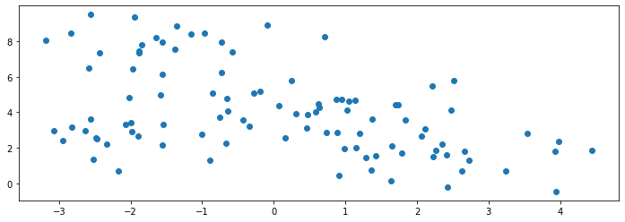
Consider the following dataset, which is generated from a mixture of four Gaussians. Below, we display 100 samples generated by the mixture distribution:
import numpy as np
from sklearn import datasets
from matplotlib import pyplot as plt
plt.rcParams['figure.figsize'] = [12, 4]

# generate 150 random points
np.random.seed(0)
X_all, y_all = datasets.make_blobs(150, centers=4)

# use the first 100 points as the main dataset
X, y = X_all[:100], y_all[:100]
plt.scatter(X[:,0], X[:,1])
<matplotlib.collections.PathCollection at 0x12b583780>
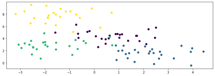
We know the true labels of these clusters, and we can visualize them with different colors as follows:
plt.scatter(X[:,0], X[:,1], c=y)
<matplotlib.collections.PathCollection at 0x115b872b0>
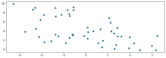
We generate another 50 datapoints to be a holdout set. We visualize them below:
# use the last 50 points as a holdout set
X_holdout, y_holdout = X_all[100:], y_all[100:]
plt.scatter(X_holdout[:,0], X_holdout[:,1])
<matplotlib.collections.PathCollection at 0x12addcf98>
10.4.2.1. Underfitting in Unsupervised Learning#
Underfitting happens when we are not able to fully learn the signal hidden in the data.
In the context of GMMs, this means not capturing all the clusters in the data.
Let’s fit a GMM on our toy dataset. Below, we define our model to be a mixture of two Gaussians and fit it to the training set:
# fit a GMM
from sklearn import mixture
model = mixture.GaussianMixture(n_components=2)
model.fit(X)
GaussianMixture(n_components=2)
The model finds two distinct components in the data, but they fail to capture the true structure.
We can also measure the value of our objective (the log-likelihood) on the training and holdout sets.
plt.scatter(X[:,0], X[:,1], c=y)
plt.scatter(model.means_[:,0], model.means_[:,1], marker='D', c='r', s=100)
print('Training Set Log-Likelihood (higher is better): %.2f' % model.score(X))
print('Holdout Set Log-Likelihood (higher is better): %.2f' % model.score(X_holdout))
Training Set Log-Likelihood (higher is better): -4.09
Holdout Set Log-Likelihood (higher is better): -4.22
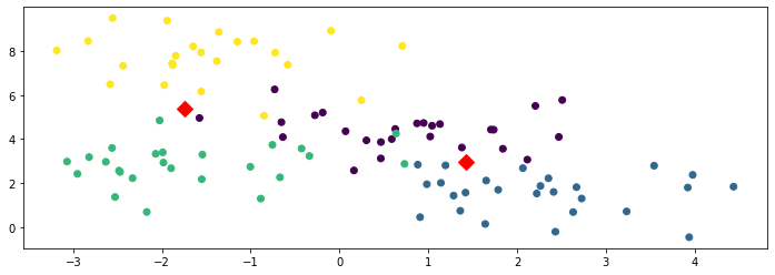
The above figure shows the learned cluster centroids as red diamonds and the training set as colored dots. You can see that the cluster centroids do not represent each class well, i.e., the model is underfitting.
10.4.2.2. Overfitting in Unsupervised Learning#
Consider now what happens if we further increase the number of clusters.
Ks = [4, 10, 20]
f, axes = plt.subplots(1,3)
for k, ax in zip(Ks, axes):
    model = mixture.GaussianMixture(n_components=k)
    model.fit(X)
    ax.scatter(X[:,0], X[:,1], c=y)
    ax.scatter(model.means_[:,0], model.means_[:,1], marker='D', c='r', s=100)
    ax.set_title('Train LL: %.2f | Holdout LL: %.2f' % (model.score(X), model.score(X_holdout)))
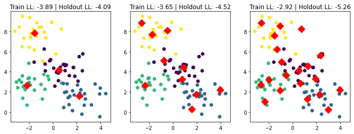
In the above figures, we can see that the leftmost figure has the best holdout set’s objective value since we define the model to be a mixture of four Gaussians. As we increase the number of clusters, though the training set objective value gets better, the holdout set objective value gets worse; this means we are overfitting.
10.4.3. Measuring Generalization Using Log-Likelihood#
Probabilistic unsupervised models optimize an objective that can be used to detect overfitting and underfitting by comparing performance between training and holdout sets.
Below, we visualize the performance (measured via negative log-likelihood) on training and holdout sets as \(K\) increases.
Ks, training_objs, holdout_objs = range(1,25), [], []
for k in Ks:
    model = mixture.GaussianMixture(n_components=k)
    model.fit(X)
    training_objs.append(-model.score(X))
    holdout_objs.append(-model.score(X_holdout))

plt.plot(Ks, training_objs, '.-', markersize=15)
plt.plot(Ks, holdout_objs, '.-', markersize=15)
plt.xlabel("Number of clusters K")
plt.ylabel("Negative Log-Likelihood")
plt.title("Training and Holdout Negative Log-Likelihood (Lower is Better)")
plt.legend(['Training Negative Log-Likelihood', 'Holdout Negative Log-Likelihood'])
<matplotlib.legend.Legend at 0x12c463320>
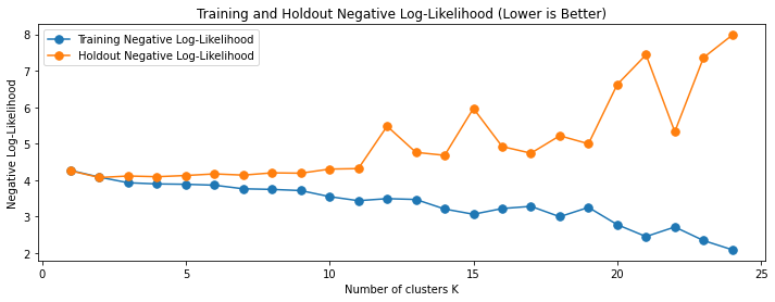
The above figure shows that when the number of clusters is below 4, adding more clusters helps reduce both training and holdout sets’ negative log-likelihood. When the number of clusters is sufficiently large, adding more clusters reduces the training set’s negative log-likelihood but increases the holdset’s negative log-likelihood. The former situation represents underfitting – you can make the model perform better on both training and holdout sets by making the model more expressive. The latter situation represents overfitting – making the model more expressive makes the performance on the holdout set worse.