Lecture 3: Linear Regression
Contents
Lecture 3: Linear Regression#
In this lecture, we will define our first supervised learning algorithm: ordinary least squares (OLS). Ordinary least squares is an algorithm for linear regression.
3.1. Calculus Review#
3.1.1. Optimization#
Recall that a key part of a supervised learning algorithm is the optimizer, which takes an objective \(J\) (also called a loss function) and a model class \(\mathcal{M}\). It outputs a model \(f \in \mathcal{M}\) with the smallest value of the objective \(J\).
Usually, this is the function that best “fits” the training dataset \(\mathcal{D} = \{(x^{(i)}, y^{(i)}) \mid i = 1,2,...,n\}\).
We will need several tools from calculus to define an optimizer.
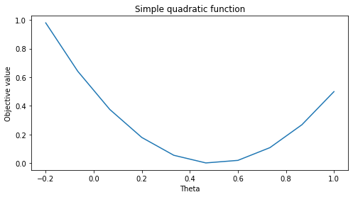
We will use the a quadratic function as our running example of an objective \(J\) in this section. Let’s define this function below.
import numpy as np
import matplotlib.pyplot as plt
plt.rcParams['figure.figsize'] = [8, 4]
def quadratic_function(theta):
    """The cost function, J(theta)."""
    return 0.5*(2*theta-1)**2
Let’s visualize this function.
# First construct a grid of theta1 parameter pairs and their corresponding
# cost function values.
thetas = np.linspace(-0.2,1,10)
f_vals = quadratic_function(thetas[:,np.newaxis])

plt.plot(thetas, f_vals)
plt.xlabel('Theta')
plt.ylabel('Objective value')
plt.title('Simple quadratic function')
Text(0.5, 1.0, 'Simple quadratic function')
3.1.2. Calculus Review: Derivatives and Gradients#
The key tool from calculus that we will use is the derivative and its extensions
Derivatives#
Recall that the derivative
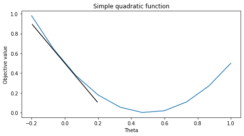
of a univariate function \(f : \mathbb{R} \to \mathbb{R}\) is the instantaneous rate of change of the function \(f(\theta)\) with respect to its parameter \(\theta\) at the point \(\theta_0\).
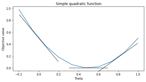
The code below visualizes several derivatives of the quadratic function. Note that the derivatives are the slopes of the tangents at various points of the curve.
def quadratic_derivative(theta):
    return (2*theta-1)*2

df0 = quadratic_derivative(np.array([[0]])) # derivative at zero
f0 = quadratic_function(np.array([[0]]))
line_length = 0.2

plt.plot(thetas, f_vals)
plt.annotate('', xytext=(0-line_length, f0-line_length*df0), xy=(0+line_length, f0+line_length*df0),
             arrowprops={'arrowstyle': '-', 'lw': 1.5}, va='center', ha='center')
plt.xlabel('Theta')
plt.ylabel('Objective value')
plt.title('Simple quadratic function')
Text(0.5, 1.0, 'Simple quadratic function')
pts = np.array([[0, 0.5, 0.8]]).reshape((3,1))
df0s = quadratic_derivative(pts)
f0s = quadratic_function(pts)

plt.plot(thetas, f_vals)
for pt, f0, df0 in zip(pts.flatten(), f0s.flatten(), df0s.flatten()):
    plt.annotate('', xytext=(pt-line_length, f0-line_length*df0), xy=(pt+line_length, f0+line_length*df0),
             arrowprops={'arrowstyle': '-', 'lw': 1}, va='center', ha='center')
plt.xlabel('Theta')
plt.ylabel('Objective value')
plt.title('Simple quadratic function')
Text(0.5, 1.0, 'Simple quadratic function')
Partial Derivatives#
The partial derivative
of a multivariate function \(f : \mathbb{R}^d \to \mathbb{R}\) is the derivative of \(f\) with respect to \(\theta_j\) while all the other dimensions \(\theta_k\) for \(k\neq j\) are fixed.
The Gradient#
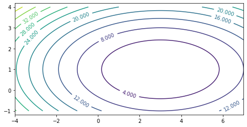
The gradient \(\nabla f\) is the vector of all the partial derivatives:
The \(j\)-th entry of the vector \(\nabla f (\theta)\) is the partial derivative \(\frac{\partial f(\theta)}{\partial \theta_j}\) of \(f\) with respect to the \(j\)-th component of \(\theta\).
We will use a quadratic function as a running example. We define this function in 2D below.
def quadratic_function2d(theta0, theta1):
    """Quadratic objective function, J(theta0, theta1).

    The inputs theta0, theta1 are 2d arrays and we evaluate
    the objective at each value theta0[i,j], theta1[i,j].
    We implement it this way so it's easier to plot the
    level curves of the function in 2d.

    Parameters:
    theta0 (np.array): 2d array of first parameter theta0
    theta1 (np.array): 2d array of second parameter theta1

    Returns:
    fvals (np.array): 2d array of objective function values
        fvals is the same dimension as theta0 and theta1.
        fvals[i,j] is the value at theta0[i,j] and theta1[i,j].
    """
    theta0 = np.atleast_2d(np.asarray(theta0))
    theta1 = np.atleast_2d(np.asarray(theta1))
    return 0.5*((2*theta1-2)**2 + (theta0-3)**2)
Let’s visualize this function. What you see below are the level curves: the value of the function is constant along each curve.
theta0_grid = np.linspace(-4,7,101)
theta1_grid = np.linspace(-1,4,101)
theta_grid = theta0_grid[np.newaxis,:], theta1_grid[:,np.newaxis]
J_grid = quadratic_function2d(theta0_grid[np.newaxis,:], theta1_grid[:,np.newaxis])

X, Y = np.meshgrid(theta0_grid, theta1_grid)
contours = plt.contour(X, Y, J_grid, 10)
plt.clabel(contours)
plt.axis('equal')
(-4.0, 7.0, -1.0, 4.0)
Let’s write down the derivative of the quadratic function.
def quadratic_derivative2d(theta0, theta1):
    """Derivative of quadratic objective function.

    The inputs theta0, theta1 are 1d arrays and we evaluate
    the derivative at each value theta0[i], theta1[i].

    Parameters:
    theta0 (np.array): 1d array of first parameter theta0
    theta1 (np.array): 1d array of second parameter theta1

    Returns:
    grads (np.array): 2d array of partial derivatives
        grads is of the same size as theta0 and theta1
        along first dimension and of size
        two along the second dimension.
        grads[i,j] is the j-th partial derivative
        at input theta0[i], theta1[i].
    """
    # this is the gradient of 0.5*((2*theta1-2)**2 + (theta0-3)**2)
    grads = np.stack([theta0-3, (2*theta1-2)*2], axis=1)
    grads = grads.reshape([len(theta0), 2])
    return grads
We can visualize the gradient. In two dimensions, the gradient can be visualized as an arrow. Note that the gradient is always orthogonal to the level curves (it’s something you prove in a Calculus 3 course).
theta0_pts, theta1_pts = np.array([2.3, -1.35, -2.3]), np.array([2.4, -0.15, 2.75])
dfs = quadratic_derivative2d(theta0_pts, theta1_pts)
line_length = 0.2

contours = plt.contour(X, Y, J_grid, 10)
for theta0_pt, theta1_pt, df0 in zip(theta0_pts, theta1_pts, dfs):
    plt.annotate('', xytext=(theta0_pt, theta1_pt),
                     xy=(theta0_pt-line_length*df0[0], theta1_pt-line_length*df0[1]),
                     arrowprops={'arrowstyle': '->', 'lw': 2}, va='center', ha='center')
plt.scatter(theta0_pts, theta1_pts)
plt.clabel(contours)
plt.xlabel('Theta0')
plt.ylabel('Theta1')
plt.title('Gradients of the quadratic function')
plt.axis('equal')
(-4.0, 7.0, -1.0, 4.0)
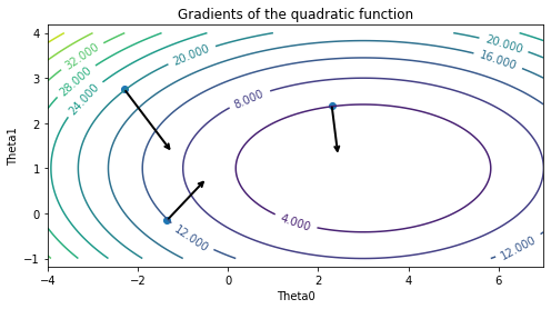
Please note that, technically, the above figure visualizes not the gradient \(\nabla J\) but its negative \(- \nabla J\), which is called the steepest descent direction.
3.1.3. Gradient Descent#
Next, we will use gradients to define an important algorithm called gradient descent.
Gradient descent is a very common optimization algorithm used in machine learning. It iteratively computes the gradient to determine the direction in which the function decreases most steeply and takes a step in that direction.
Notation#
More formally, if we want to optimize \(J(\theta)\), we start with an initial guess \(\theta_0\) for the parameters and repeat the following update until \(\theta\) is no longer changing:
In pseudocode, this method may look as follows:
theta, theta_prev = random_initialization()
while norm(theta - theta_prev) > convergence_threshold:
    theta_prev = theta
    theta = theta_prev - step_size * gradient(theta_prev)
In the above algorithm, we stop when \(||\theta_i - \theta_{i-1}||\) is small.
It’s easy to implement this function in numpy.
convergence_threshold = 2e-1
step_size = 2e-1
theta, theta_prev = np.array([[-2], [3]]), np.array([[0], [0]])
opt_pts = [theta.flatten()]
opt_grads = []

while np.linalg.norm(theta - theta_prev) > convergence_threshold:
    # we repeat this while the value of the function is decreasing
    theta_prev = theta
    gradient = quadratic_derivative2d(*theta).reshape([2,1])
    theta = theta_prev - step_size * gradient
    # also, record the points visited by gradient descent and their gradients
    opt_pts += [theta.flatten()]
    opt_grads += [gradient.flatten()]
Let’s run gradient descent and visualize its trajectory by displaying the points visited over the course of the optimization procedure.
opt_pts = np.array(opt_pts)
opt_grads = np.array(opt_grads)

contours = plt.contour(X, Y, J_grid, 10)
plt.clabel(contours)
plt.scatter(opt_pts[:,0], opt_pts[:,1])

for opt_pt, opt_grad in zip(opt_pts, opt_grads):
    plt.annotate('', xytext=(opt_pt[0], opt_pt[1]),
                 xy=(opt_pt[0]-0.8*step_size*opt_grad[0], opt_pt[1]-0.8*step_size*opt_grad[1]),
                 arrowprops={'arrowstyle': '->', 'lw': 2}, va='center', ha='center')

plt.axis('equal')
(-4.0, 7.0, -1.0, 4.0)
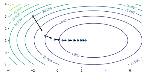
Each gradient is orthogonal to the level curve, and the direction opposite to gradient (the “steepest descent direction”, shown by arrows on the above figure) points inwards toward the minimum. By repeatedly following the steepest descent direction, we arrive at the minimum.
3.2. Gradient Descent in Linear Models#
We can use gradient descent as the basis of our first supervised learning algorithm. Note that this will be a toy algorithm: in practice there exists a better way than gradient descent to optimize the learning objective of a linear model. We will see it in the next section.
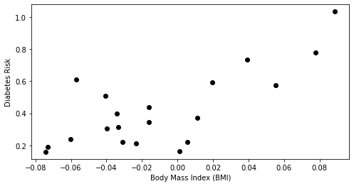
3.2.1. A Supervised Learning Task: Predicting Diabetes#
In this section, we are going to again use the UCI Diabetes Dataset.
For each patient we have a access to their BMI and an estimate of diabetes risk (from 0-400).
We are interested in understanding how BMI affects an individual’s diabetes risk.
%matplotlib inline
import matplotlib.pyplot as plt
plt.rcParams['figure.figsize'] = [8, 4]

import numpy as np
import pandas as pd
from sklearn import datasets

# Load the diabetes dataset
X, y = datasets.load_diabetes(return_X_y=True, as_frame=True)

# add an extra column of onens
X['one'] = 1

# Collect 20 data points and only use bmi dimension
X_train = X.iloc[-20:].loc[:, ['bmi', 'one']]
y_train = y.iloc[-20:] / 300

plt.scatter(X_train.loc[:,['bmi']], y_train,  color='black')
plt.xlabel('Body Mass Index (BMI)')
plt.ylabel('Diabetes Risk')
Text(0, 0.5, 'Diabetes Risk')
3.2.2. Linear Model Family#
Recall that a linear model has the form
where \(x \in \mathbb{R}^d\) is a vector of features and \(y\) is the target. The \(\theta_j\) are the parameters of the model.
By using the notation \(x_0 = 1\), we can represent the model in a more compact vectorized form
Let’s define our model in Python.
def f(X, theta):
    """The linear model we are trying to fit.

    Parameters:
    theta (np.array): d-dimensional vector of parameters
    X (np.array): (n,d)-dimensional data matrix

    Returns:
    y_pred (np.array): n-dimensional vector of predicted targets
    """
    return X.dot(theta)
3.2.3. An Objective: Mean Squared Error#
We pick \(\theta\) to minimize the mean squared error (MSE). Slightly different versions of this objective are also known as the residual sum of squares (RSS) or the sum of squared residuals (SSR).
In other words, by minimizing this objective, we are trying to find \(\theta\) such that the predictions \(\theta^\top x^{(i)}\) are as close as possible to the targets \(y^{(i)}\).
Let’s implement the mean squared error.
def mean_squared_error(theta, X, y):
    """The cost function, J, describing the goodness of fit.

    Parameters:
    theta (np.array): d-dimensional vector of parameters
    X (np.array): (n,d)-dimensional design matrix
    y (np.array): n-dimensional vector of targets
    """
    return 0.5*np.mean((y-f(X, theta))**2)
Mean Squared Error: Derivatives and Gradients#
Let’s work out the derivatives for \(\frac{1}{2} \left( f_\theta(x^{(i)}) - y^{(i)} \right)^2,\) the MSE of a linear model \(f_\theta\) for one training example \((x^{(i)}, y^{(i)})\), which we denote \(J^{(i)}(\theta)\).
We can use this derivation to obtain an expression for the gradient of the MSE for a linear model
Note that the MSE over the entire dataset is \(J(\theta) = \frac{1}{n}\sum_{i=1}^n J^{(i)}(\theta)\). Therefore:
Let’s implement this gradient.
def mse_gradient(theta, X, y):
    """The gradient of the cost function.

    Parameters:
    theta (np.array): d-dimensional vector of parameters
    X (np.array): (n,d)-dimensional design matrix
    y (np.array): n-dimensional vector of targets

    Returns:
    grad (np.array): d-dimensional gradient of the MSE
    """
    return np.mean((f(X, theta) - y) * X.T, axis=1)
3.2.4. Gradient Descent for Linear Regression#
Plugging in the above gradient into the gradient descent algorithm, we obtain a learning method for training linear models.
theta, theta_prev = random_initialization()
while abs(J(theta) - J(theta_prev)) > conv_threshold:
    theta_prev = theta
    theta = theta_prev - step_size * (f(x, theta)-y) * x
This update rule is also known as the Least Mean Squares (LMS) or Widrow-Hoff learning rule.
threshold = 1e-3
step_size = 4e-1
theta, theta_prev = np.array([2,1]), np.ones(2,)
opt_pts = [theta]
opt_grads = []
iter = 0

while np.linalg.norm(theta - theta_prev) > threshold:
    if iter % 100 == 0:
        print('Iteration %d. MSE: %.6f' % (iter, mean_squared_error(theta, X_train, y_train)))
    theta_prev = theta
    gradient = mse_gradient(theta, X_train, y_train)
    theta = theta_prev - step_size * gradient
    opt_pts += [theta]
    opt_grads += [gradient]
    iter += 1
Iteration 0. MSE: 0.171729
Iteration 100. MSE: 0.014765
Iteration 200. MSE: 0.014349
Iteration 300. MSE: 0.013997
Iteration 400. MSE: 0.013701
This procedure yields a first concrete example of a supervised learning algorithm. The final weights returned by the above algorithm yield a model, which we can visualize below.
x_line = np.stack([np.linspace(-0.1, 0.1, 10), np.ones(10,)])
y_line = opt_pts[-1].dot(x_line)

plt.scatter(X_train.loc[:,['bmi']], y_train,  color='black')
plt.plot(x_line[0], y_line)
plt.xlabel('Body Mass Index (BMI)')
plt.ylabel('Diabetes Risk')
Text(0, 0.5, 'Diabetes Risk')
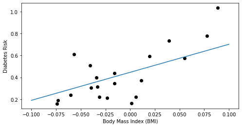
Note that the result is similar to what we obtained in the previous lecture by invoking the optimizer in scikit-learn.
3.3. Ordinary Least Squares#
In practice, there is a better way to find linear model parameters that does not rely on gradient descent. This method will produce our first non-toy supervised learning algorithm: Ordinary Least Squares.
3.3.1. Notation#
First, we start by introducing some notation. Suppose that we have a dataset of size \(n\) (e.g., \(n\) patients), indexed by \(i=1,2,...,n\). Each \(x^{(i)}\) is a vector of \(d\) features.
Design Matrix#
Machine learning algorithms are most easily defined in the language of linear algebra. Therefore, it will be useful to represent the entire dataset as one matrix \(X \in \mathbb{R}^{n \times d}\), of the form:
Let’s print out the design matrix for the diabetes dataset.
X_train.head()
| age | sex | bmi | bp | s1 | s2 | s3 | s4 | s5 | s6 | one | |
|---|---|---|---|---|---|---|---|---|---|---|---|
| 422 | -0.078165 | 0.050680 | 0.077863 | 0.052858 | 0.078236 | 0.064447 | 0.026550 | -0.002592 | 0.040672 | -0.009362 | 1 |
| 423 | 0.009016 | 0.050680 | -0.039618 | 0.028758 | 0.038334 | 0.073529 | -0.072854 | 0.108111 | 0.015567 | -0.046641 | 1 |
| 424 | 0.001751 | 0.050680 | 0.011039 | -0.019442 | -0.016704 | -0.003819 | -0.047082 | 0.034309 | 0.024053 | 0.023775 | 1 |
| 425 | -0.078165 | -0.044642 | -0.040696 | -0.081414 | -0.100638 | -0.112795 | 0.022869 | -0.076395 | -0.020289 | -0.050783 | 1 |
| 426 | 0.030811 | 0.050680 | -0.034229 | 0.043677 | 0.057597 | 0.068831 | -0.032356 | 0.057557 | 0.035462 | 0.085907 | 1 |
The Target Vector#
Similarly, we can vectorize the target variables into a vector \(y \in \mathbb{R}^n\) of the form
Squared Error in Matrix Form#
We may fit a linear model by choosing \(\theta\) that minimizes the sum of squares error.
We can write this sum in matrix-vector form as:
where \(X\) is the design matrix and \(\|\cdot\|\) denotes the Euclidean norm.
3.3.2. The Normal Equations#
Next, we will use this notation to derive a very important formula in supervised learning—the normal equations.
The Gradient of the Squared Error#
Let’s begin by observing that we can compute the gradient of the mean squared error as follows.
We used the facts that \(a^\top b = b^\top a\) (line 3), that \(\nabla_x b^\top x = b\) (line 4), and that \(\nabla_x x^\top A x = 2 A x\) for a symmetric matrix \(A\) (line 4).
Computing Model Parameters via the Normal Equations#
We know from calculus that a function is minimized when its derivative is set to zero. In our case, our objective function is a (multivariate) quadratic; hence it only has one minimum, which is the global minimum.
Setting the above derivative to zero, we obtain the normal equations:
Hence, the value \(\theta^*\) that minimizes this objective is given by:
Note that we assumed that the matrix \((X^\top X)\) is invertible; we will soon see a simple way of dealing with non-invertible matrices.
We also add a few important remarks:
The formula \(\theta^* = (X^\top X)^{-1} X^\top y\) yields an analytical formula for the parameters that minimize our mean squared error objective.
In contrast, gradient descent is an iterative optimization procedure that is often slower on small datasets.
The analytical approach is what is most commonly used in practice.
Example: OLS on the Diabetes dataset#
Let’s now apply the normal equations to the Diabetes dataset.
import numpy as np

theta_best = np.linalg.inv(X_train.T.dot(X_train)).dot(X_train.T).dot(y_train)
theta_best_df = pd.DataFrame(data=theta_best[np.newaxis, :], columns=X.columns)
theta_best_df
| age | sex | bmi | bp | s1 | s2 | s3 | s4 | s5 | s6 | one | |
|---|---|---|---|---|---|---|---|---|---|---|---|
| 0 | -3.888868 | 204.648785 | -64.289163 | -262.796691 | 14003.726808 | -11798.307781 | -5892.15807 | -1136.947646 | -2736.597108 | -393.879743 | 155.698998 |
The above dataframe contains the parameters that minimize the mean squared error objective.
We can now use our estimate of theta to compute predictions for 3 new data points.
# Collect 3 data points for testing
X_test = X.iloc[:3]
y_test = y.iloc[:3]

# generate predictions on the new patients
y_test_pred = X_test.dot(theta_best)
Let’s visualize these predictions.
# visualize the results
plt.xlabel('Body Mass Index (BMI)')
plt.ylabel('Diabetes Risk')
plt.scatter(X_train.loc[:, ['bmi']], y_train)
plt.scatter(X_test.loc[:, ['bmi']], y_test, color='red', marker='o')
plt.plot(X_test.loc[:, ['bmi']], y_test_pred, 'x', color='red', mew=3, markersize=8)
plt.legend(['Model', 'Prediction', 'Initial patients', 'New patients'])
<matplotlib.legend.Legend at 0x128d89668>
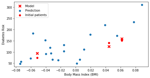
Again, red crosses denote predictions; red dots are true values. The model gives us very accurate predictions.
Recall again that although we are visualizing the data with the BMI on the x-axis, the model actually uses all of the features for its predictions.
3.3.4. Ordinary Least Squares#
The above procedure gives us our first non-toy supervised learning algorithm—ordinary least squares (OLS). We can succinctly define OLS in terms of the algorithm components we defined in the last lecture.
Type: Supervised learning (regression)
Model family: Linear models
Objective function: Mean squared error
Optimizer: Normal equations
We will define many algorithms in this way throughout the course.
3.4. Non-Linear Least Squares#
Ordinary Least Squares can only learn linear relationships in the data. Can we also use it to model more complex relationships?
3.4.1. Review: Polynomial Functions#
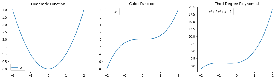
We start with a brief review of polynomials. Recall that a polynomial of degree \(p\) is a function of the form
Below are some examples of polynomial functions.
import warnings
warnings.filterwarnings("ignore")

plt.figure(figsize=(16,4))
x_vars = np.linspace(-2, 2)

plt.subplot('131')
plt.title('Quadratic Function')
plt.plot(x_vars, x_vars**2)
plt.legend(["$x^2$"])

plt.subplot('132')
plt.title('Cubic Function')
plt.plot(x_vars, x_vars**3)
plt.legend(["$x^3$"])

plt.subplot('133')
plt.title('Third Degree Polynomial')
plt.plot(x_vars, x_vars**3 + 2*x_vars**2 + x_vars + 1)
plt.legend(["$x^3 + 2 x^2 + x + 1$"])
<matplotlib.legend.Legend at 0x128ed2ac8>
3.4.2. Modeling Non-Linear Relationships With Polynomial Regression#
Note that the set of \(p\)-th degree polynomials forms a linear model with parameters \(a_p, a_{p-1}, ..., a_0\). This means we can use our algorithms for linear models to learn non-linear features!
Specifically, given a one-dimensional continuous variable \(x\), we can define the polynomial feature function \(\phi : \mathbb{R} \to \mathbb{R}^{p+1}\) as
The class of models of the form
with parameters \(\theta\) and polynomial features \(\phi\) is the set of \(p\)-degree polynomials.
This model is non-linear in the input variable \(x\), meaning that we can model complex data relationships.
It is a linear model as a function of the parameters \(\theta\), meaning that we can use our familiar ordinary least squares algorithm to learn these features.
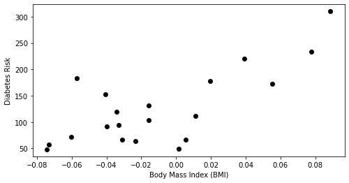
Polynomial Features for Diabetes RIsk Prediction#
In this section, we are going to again load the UCI Diabetes Dataset. Recall that:
For each patient we have a access to a measurement of their body mass index (BMI) and a quantitative diabetes risk score (from 0-300).
We are interested in understanding how BMI affects an individual’s diabetes risk.
%matplotlib inline
import matplotlib.pyplot as plt
plt.rcParams['figure.figsize'] = [8, 4]

import numpy as np
import pandas as pd
from sklearn import datasets

# Load the diabetes dataset
X, y = datasets.load_diabetes(return_X_y=True, as_frame=True)

# add an extra column of onens
X['one'] = 1

# Collect 20 data points
X_train = X.iloc[-20:]
y_train = y.iloc[-20:]

plt.scatter(X_train.loc[:,['bmi']], y_train,  color='black')
plt.xlabel('Body Mass Index (BMI)')
plt.ylabel('Diabetes Risk')
Text(0, 0.5, 'Diabetes Risk')
Let’s now obtain linear features for this dataset.
X_bmi = X_train.loc[:, ['bmi']]

X_bmi_p3 = pd.concat([X_bmi, X_bmi**2, X_bmi**3], axis=1)
X_bmi_p3.columns = ['bmi', 'bmi2', 'bmi3']
X_bmi_p3['one'] = 1
X_bmi_p3.head()
| bmi | bmi2 | bmi3 | one | |
|---|---|---|---|---|
| 422 | 0.077863 | 0.006063 | 0.000472 | 1 |
| 423 | -0.039618 | 0.001570 | -0.000062 | 1 |
| 424 | 0.011039 | 0.000122 | 0.000001 | 1 |
| 425 | -0.040696 | 0.001656 | -0.000067 | 1 |
| 426 | -0.034229 | 0.001172 | -0.000040 | 1 |
Diabetes RIsk Prediction with Polynomial Regression#
By training a linear model on this featurization of the diabetes dataset, we obtain a polynomial model of diabetes risk as a function of BMI.
# Fit a linear regression
theta = np.linalg.inv(X_bmi_p3.T.dot(X_bmi_p3)).dot(X_bmi_p3.T).dot(y_train)

# Show the learned polynomial curve
x_line = np.linspace(-0.1, 0.1, 10)
x_line_p3 = np.stack([x_line, x_line**2, x_line**3, np.ones(10,)], axis=1)
y_train_pred = x_line_p3.dot(theta)

plt.xlabel('Body Mass Index (BMI)')
plt.ylabel('Diabetes Risk')
plt.scatter(X_bmi, y_train)
plt.plot(x_line, y_train_pred)
[<matplotlib.lines.Line2D at 0x1292c99e8>]
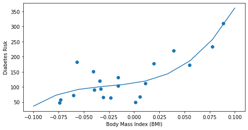
Notice how the above third-degree polynomial represents a much better fit to the data.
3.4.3. Multivariate Polynomial Regression#
We can construct non-linear functions of multiple variables by using multivariate polynomials. For example, a polynomial of degree \(2\) over two variables \(x_1, x_2\) is a function of the form
In general, a polynomial of degree \(p\) over two variables \(x_1, x_2\) is a function of the form $\( f(x_1, x_2) = \sum_{i,j \geq 0 : i+j \leq p} a_{ij} x_1^i x_2^j. \)$
In our two-dimensional example, this corresponds to a feature function \(\phi : \mathbb{R}^2 \to \mathbb{R}^6\) of the form
The same approach can be used to specify polynomials of any degree and over any number of variables.
3.4.4. Non-Linear Least Squares#
We can further extend this approach by going from polynomial to general non-linear features. Combining non-linear features with normal equations gives us an algorithm called non-linear least squares.
Towards General Non-Linear Features#
Any non-linear feature map \(\phi(x) : \mathbb{R}^d \to \mathbb{R}^p\) can be used to obtain general models of the form
that are highly non-linear in \(x\) but linear in \(\theta\).
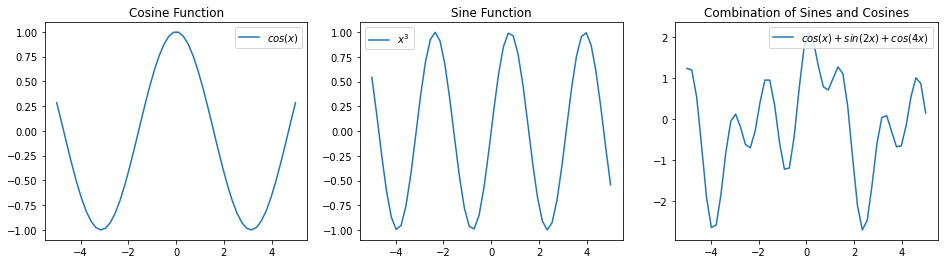
For example, here is a way of modeling complex periodic functions via a sum of sines and cosines.
import warnings
warnings.filterwarnings("ignore")

plt.figure(figsize=(16,4))
x_vars = np.linspace(-5, 5)

plt.subplot('131')
plt.title('Cosine Function')
plt.plot(x_vars, np.cos(x_vars))
plt.legend(["$cos(x)$"])

plt.subplot('132')
plt.title('Sine Function')
plt.plot(x_vars, np.sin(2*x_vars))
plt.legend(["$x^3$"])

plt.subplot('133')
plt.title('Combination of Sines and Cosines')
plt.plot(x_vars, np.cos(x_vars) + np.sin(2*x_vars) + np.cos(4*x_vars))
plt.legend(["$cos(x) + sin(2x) + cos(4x)$"])
<matplotlib.legend.Legend at 0x129571160>
Algorithm: Non-Linear Least Squares#
Because the above model is still linear in \(\theta\), we can apply the normal equations. This yields the following algorithm, which we again characterize via its components.
Type: Supervised learning (regression)
Model family: Linear in the parameters; non-linear with respect to raw inputs.
Features: Non-linear functions of the attributes
Objective function: Mean squared error
Optimizer: Normal equations