Lecture 2: Supervised Machine Learning

This lecture will dive deeper into supervised learning and introduce mathematical notation that will be useful throughout the course.

2.1. Elements of A Supervised Machine Learning Problem

Let’s first look at a more detailed example of a supervised learning problem. We will use a simple running example—predicting the diabetes risk of a patient from their BMI.

Three Components of Supervised Machine Learning

It is useful to think of supervised learning as involving three key elements: a dataset, a learning algorithm, and a predictive model.

To apply supervised learning, we define a dataset and a learning algorithm.

\[ \text{Dataset} + \text{Learning Algorithm} \to \text{Predictive Model} \]

The result of running the learning algorithm on the dataset is a predictive model that maps inputs to targets. For instance, it can predict targets on new inputs. Next, we will give examples of each of these three components.

2.1.1. A Supervised Learning Dataset

Let’s start with a simple dataset of medical patients.

• For each patient we have a access to their BMI and an estimate of diabetes risk (from 0-400).

• We are interested in understanding how BMI affects an individual’s diabetes risk.

We are going to load a real diabetes dataset from scikit-learn, a popular machine learning library that we will use throughout the course.

import numpy as np
import pandas as pd
from sklearn import datasets

# We will use the UCI Diabetes Dataset
# It's a toy dataset often used to demo ML algorithms.
diabetes_X, diabetes_y = datasets.load_diabetes(return_X_y=True, as_frame=True)

# Use only the BMI feature
diabetes_X = diabetes_X.loc[:, ['bmi']]

# The BMI is zero-centered and normalized; we recenter it for ease of presentation
diabetes_X = diabetes_X * 30 + 25

# Collect 20 data points
diabetes_X_train = diabetes_X.iloc[-20:]
diabetes_y_train = diabetes_y.iloc[-20:]

# Display some of the data points
pd.concat([diabetes_X_train, diabetes_y_train], axis=1).head()

	bmi	target
422	27.335902	233.0
423	23.811456	91.0
424	25.331171	111.0
425	23.779122	152.0
426	23.973128	120.0

Let’s also visualize this two-dimensional dataset.

%matplotlib inline
import matplotlib.pyplot as plt
plt.rcParams['figure.figsize'] = [12, 4]

plt.scatter(diabetes_X_train, diabetes_y_train,  color='black')
plt.xlabel('Body Mass Index (BMI)')
plt.ylabel('Diabetes Risk')

Text(0, 0.5, 'Diabetes Risk')

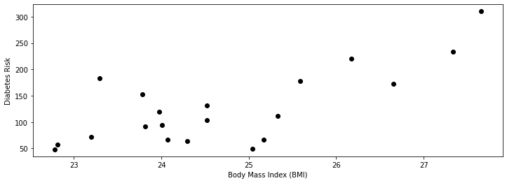
We see from the above figure that diabetes risk grows as the patient’s BMI increases.

2.1.2. A Supervised Learning Algorithm

Next, suppose we wanted to predict the risk of a new patient given their BMI. It will be useful to think about a supervised learning algorithm as having two components: a model class and an optimizer.

The Model Class

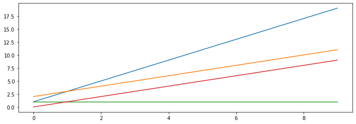
Intuitively, the model class represents the set of possible relationships between BMI and risk that we believe to be true. Let’s assume in this example that risk is a linear function of BMI. In other words, for some unknown \(\theta_0, \theta_1 \in \mathbb{R}\), we have

\[ y = \theta_1 \cdot x + \theta_0, \]

where \(x\) is the BMI (also called the independent variable), and \(y\) is the diabetes risk score (the dependent variable). The parameters \(\theta_1, \theta_0\) are the slope and the intercept of the line relates \(x\) to \(y\).

We can visualize this for a few values of \(\theta_1, \theta_0\).

theta_list = [(1, 2), (2,1), (1,0), (0,1)]
for theta0, theta1 in theta_list:
    x = np.arange(10)
    y = theta1 * x + theta0
    plt.plot(x,y)

Our supervised learning algorithm will attempt to choose the linear relationship fits the training data well.

The Optimizer

Given our assumption that \(x,y\) follow a linear relationship, the goal of a supervised learning algorithm is to find a good set of parameters consistent with the data.

This is an optimization problem—we want to maximize the fit between the model and the data over the space of all possible models. The component of a supervised learning algorithm that performs this search procedure is called the optimizer.

We will soon dive deeper into optimization algorithms for machine learning, but for now, let’s call the sklearn.linear_model library to find a \(\theta_1, \theta_0\) that fit the data well.

from sklearn import linear_model
from sklearn.metrics import mean_squared_error

# Create linear regression object
regr = linear_model.LinearRegression()

# Train the model using the training sets
regr.fit(diabetes_X_train, diabetes_y_train.values)

# Make predictions on the training set
diabetes_y_train_pred = regr.predict(diabetes_X_train)

# The coefficients
print('Slope (theta1): \t', regr.coef_[0])
print('Intercept (theta0): \t', regr.intercept_)

Slope (theta1): 	 37.378842160517664
Intercept (theta0): 	 -797.0817390342369

Here, we used scikit-learn to find the best slope and intercept to the above dataset.

2.1.3. A Supervised Learning Model

The supervised learning algorithm gave us a pair of parameters \(\theta_1^*, \theta_0^*\). These define the predictive model \(f\), defined as

\[ f(x) = \theta_1^* \cdot x + \theta_0^*, \]

where again \(x\) is the BMI, and \(y\) is the diabetes risk score.

We can visualize the linear model that best fits our data.

plt.xlabel('Body Mass Index (BMI)')
plt.ylabel('Diabetes Risk')
plt.scatter(diabetes_X_train, diabetes_y_train)
plt.plot(diabetes_X_train, diabetes_y_train_pred, color='black', linewidth=2)

[<matplotlib.lines.Line2D at 0x1253f9240>]

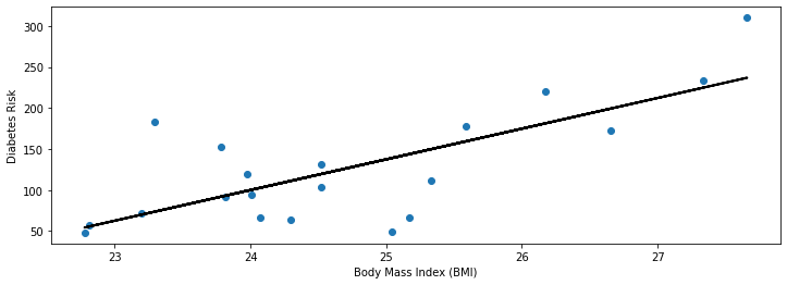
Our visualization seems reasonable: we see that the linear model that we found is close to the observed data and captures the trend we noticed earlier—higher BMIs are associated with higher diabetes risk.

2.1.4. Making New Predictions

Recall that one of the goals of supervised learning is to predict diabetes risk for new patients. Given a new dataset of patients with a known BMI, we can use the predictive model to estimate their risk.

Formally, given an \(x_\text{new}\), we can output prediction \(y_\text{new}\) as

\[ y_\text{new} = f(x_\text{new}) = \theta_1^* \cdot x_\text{new} + \theta_0^*. \]

Let’s illustrate this equation with a specific example from our diabetes dataset.

First, we start by loading more data. We will load three new patients (shown in red below) that we haven’t seen before.

# Collect 3 data points
diabetes_X_test = diabetes_X.iloc[:3]
diabetes_y_test = diabetes_y.iloc[:3]

plt.scatter(diabetes_X_train, diabetes_y_train)
plt.scatter(diabetes_X_test, diabetes_y_test,  color='red')
plt.xlabel('Body Mass Index (BMI)')
plt.ylabel('Diabetes Risk')
plt.legend(['Initial patients', 'New patients'])

<matplotlib.legend.Legend at 0x1259cd390>

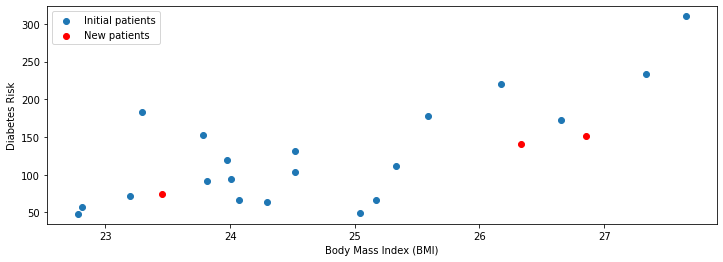
Our linear model provides an estimate of the diabetes risk for these patients.

# generate predictions on the new patients
diabetes_y_test_pred = regr.predict(diabetes_X_test)

# visualize the results
plt.xlabel('Body Mass Index (BMI)')
plt.ylabel('Diabetes Risk')
plt.scatter(diabetes_X_train, diabetes_y_train)
plt.scatter(diabetes_X_test, diabetes_y_test, color='red', marker='o')
plt.plot(diabetes_X_train, diabetes_y_train_pred, color='black', linewidth=1)
plt.plot(diabetes_X_test, diabetes_y_test_pred, 'x', color='red', mew=3, markersize=8)
plt.legend(['Model', 'Prediction', 'Initial patients', 'New patients'])

<matplotlib.legend.Legend at 0x125bfb048>

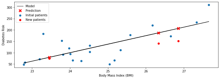
For each patient, we look up their BMI \(x\) and compute the value \(f(x)\) of the linear model \(f\) at \(x\). On the above figure, \(f(x)\) is denoted by a red cross.

We can compare the predicted value of \(f(x)\) to the known true risk \(y\) (which the model didn’t see, and which is denoted by a red circle). The model is especially accurate on the leftmost patient: the prediction \(f(x)\) and the true \(y\) almost overlap. The model is somewhat off on the other two points—however, it still correctly identifies them as being at a higher risk.

2.1.5 Why Supervised Learning?

We have just seen a simple example of a supervised learning algorithm. Again, we want to emphasize that supervised learning is a tool that is applicable on tasks such as:

• Predictive modeling. As we gather more data to characterize a patient (their age, gender, historical blood pressure, medical notes, etc), supervised learning can often outperform even human experts.

• Understanding the mechanisms through which input variables affect targets. Instead of using the predictions from the model, we may investigate the model itself. In the above example, we inspected the slope of the model, and noted that it was positive. Thus, we have inferred from data that a high BMI tends to increase diabetes risk.

More generally, supervised learning finds applications in many areas. In fact, many of the most important applications of machine learning are supervised:

• Classifying medical images. Similarly to how we predicted risk of BMI we may, for example, predict the severity of a cancer tumor from its image.

• Translating between pairs of languages. Most machine translation systems these days are created by training a supervised learning model on large datasets consisting of pairs of sentences in different languages.

• Detecting objects in a self-driving car. Again, we can explain to an algorithm what defines a car by providing many examples of cars. This enables the algorithm to detect new cars.

We will see many more examples in this course.

2.2. Anatomy of a Supervised Learning Problem: The Dataset

Let’s now examine more closely the components of a supervised learning problem, starting with the dataset.

2.2.1. What is a Supervised Learning Dataset?

We will again use the UCI Diabetes Dataset as our running example.

The UCI dataset contains many additional data columns besides bmi, including age, sex, and blood pressure. We can ask sklearn to give us more information about this dataset.

import numpy as np
import pandas as pd
import matplotlib.pyplot as plt
plt.rcParams['figure.figsize'] = [12, 4]
from sklearn import datasets

# Load the diabetes dataset
diabetes = datasets.load_diabetes(as_frame=True)
print(diabetes.DESCR)

.. _diabetes_dataset:

Diabetes dataset
----------------

Ten baseline variables, age, sex, body mass index, average blood
pressure, and six blood serum measurements were obtained for each of n =
442 diabetes patients, as well as the response of interest, a
quantitative measure of disease progression one year after baseline.

**Data Set Characteristics:**

  :Number of Instances: 442

  :Number of Attributes: First 10 columns are numeric predictive values

  :Target: Column 11 is a quantitative measure of disease progression one year after baseline

  :Attribute Information:
      - age     age in years
      - sex
      - bmi     body mass index
      - bp      average blood pressure
      - s1      tc, T-Cells (a type of white blood cells)
      - s2      ldl, low-density lipoproteins
      - s3      hdl, high-density lipoproteins
      - s4      tch, thyroid stimulating hormone
      - s5      ltg, lamotrigine
      - s6      glu, blood sugar level

Note: Each of these 10 feature variables have been mean centered and scaled by the standard deviation times `n_samples` (i.e. the sum of squares of each column totals 1).

Source URL:
https://www4.stat.ncsu.edu/~boos/var.select/diabetes.html

For more information see:
Bradley Efron, Trevor Hastie, Iain Johnstone and Robert Tibshirani (2004) "Least Angle Regression," Annals of Statistics (with discussion), 407-499.
(https://web.stanford.edu/~hastie/Papers/LARS/LeastAngle_2002.pdf)

2.2.2. A Supervised Learning Dataset: Notation

We say that a training dataset of size \(n\) (e.g., \(n\) patients) is a set

\[ \mathcal{D} = \{(x^{(i)}, y^{(i)}) \mid i = 1,2,...,n\}\]

Each \(x^{(i)}\) denotes an input (e.g., the measurements for patient \(i\)), and each \(y^{(i)} \in \mathcal{Y}\) is a target (e.g., the diabetes risk). You may think of \(x^{(i)}\) as a column vector containing numbers useful for predicting \(y^{(i)}\).

Together, \((x^{(i)}, y^{(i)})\) form a training example.

We can look at the diabetes dataset in this form.

# Load the diabetes dataset
diabetes_X, diabetes_y = diabetes.data, diabetes.target

# Print part of the dataset
diabetes_X.head()

	age	sex	bmi	bp	s1	s2	s3	s4	s5	s6
0	0.038076	0.050680	0.061696	0.021872	-0.044223	-0.034821	-0.043401	-0.002592	0.019908	-0.017646
1	-0.001882	-0.044642	-0.051474	-0.026328	-0.008449	-0.019163	0.074412	-0.039493	-0.068330	-0.092204
2	0.085299	0.050680	0.044451	-0.005671	-0.045599	-0.034194	-0.032356	-0.002592	0.002864	-0.025930
3	-0.089063	-0.044642	-0.011595	-0.036656	0.012191	0.024991	-0.036038	0.034309	0.022692	-0.009362
4	0.005383	-0.044642	-0.036385	0.021872	0.003935	0.015596	0.008142	-0.002592	-0.031991	-0.046641

In this example, each row \(i\) contains the vector \((x^{(i)})^\top\).

Note that some numbers are unusual (e.g., age is negative). This is because scikit-learn normalized this data to have mean zero and standard deviation one.

2.2.3. Training Dataset: Inputs

More precisely, an input \(x^{(i)} \in \mathcal{X}\) is a \(d\)-dimensional vector of the form

\[\begin{split} x^{(i)} = \begin{bmatrix} x^{(i)}_1 \\ x^{(i)}_2 \\ \vdots \\ x^{(i)}_d \end{bmatrix}\end{split}\]

For example, \(x^{(i)}\) could be vector of attributes describing patient \(i\). One of these attributes could be their BMI.

The set \(\mathcal{X}\) is called the feature space. Often, we have, \(\mathcal{X} = \mathbb{R}^d\).

Let’s look at data for one patient.

diabetes_X.iloc[0]

age    0.038076
sex    0.050680
bmi    0.061696
bp     0.021872
s1    -0.044223
s2    -0.034821
s3    -0.043401
s4    -0.002592
s5     0.019908
s6    -0.017646
Name: 0, dtype: float64

This indeed looks like a column vector.

Attributes

We refer to the numerical variables describing the patient as attributes. Examples of attributes include:

• The age of a patient.

• The patient’s gender.

• The patient’s BMI.

In other applications of machine learning, a vector of attributes \(x\) could be comprised of all the pixel values of an image or it could contain indicator variables for whether certain words are present or absent in an input sentence.

Features

Often, an input object has many attributes, and we want to use these attributes to define more complex characteristics of the input.

• Is the patient old and a man? (Useful if old men are at risk).

• Is the BMI above the obesity threshold?

We call these custom attributes features.

Let’s create an “old man” feature.

diabetes_X['old_man'] = (diabetes_X['sex'] > 0) & (diabetes_X['age'] > 0.05)
diabetes_X.head()

	age	sex	bmi	bp	s1	s2	s3	s4	s5	s6	old_man
0	0.038076	0.050680	0.061696	0.021872	-0.044223	-0.034821	-0.043401	-0.002592	0.019908	-0.017646	False
1	-0.001882	-0.044642	-0.051474	-0.026328	-0.008449	-0.019163	0.074412	-0.039493	-0.068330	-0.092204	False
2	0.085299	0.050680	0.044451	-0.005671	-0.045599	-0.034194	-0.032356	-0.002592	0.002864	-0.025930	True
3	-0.089063	-0.044642	-0.011595	-0.036656	0.012191	0.024991	-0.036038	0.034309	0.022692	-0.009362	False
4	0.005383	-0.044642	-0.036385	0.021872	0.003935	0.015596	0.008142	-0.002592	-0.031991	-0.046641	False

Formally, we may denote features via a function \(\phi : \mathcal{X} \to \mathbb{R}^p\) that takes an input \(x^{(i)} \in \mathcal{X}\) and outputs a \(p\)-dimensional vector

\[\begin{split} \phi(x^{(i)}) = \left[\begin{array}{@{}c@{}} \phi(x^{(i)})_1 \\ \phi(x^{(i)})_2 \\ \vdots \\ \phi(x^{(i)})_p \end{array} \right] \end{split}\]

We say that \(\phi(x^{(i)})\) is a featurized input, and each \(\phi(x^{(i)})_j\) is a feature.

Features vs Attributes

In practice, the terms attribute and features are often used interchangeably. Most authors refer to \(x^{(i)}\) as a vector of features. We will follow this convention and use the term “attribute” only when there is ambiguity between features and attributes.

Features: Discrete vs. Continuous

Features can be either discrete or continuous. We will see that some ML algorithms handle these differently.

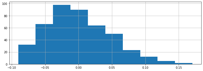
The BMI feature that we have seen earlier is an example of a continuous feature. We can visualize its distribution.

diabetes_X.loc[:, 'bmi'].hist()

<AxesSubplot:>

Other features take on one of a finite number of discrete values. The sex column is an example of a categorical feature.

print(diabetes_X.loc[:, 'sex'].unique())
diabetes_X.loc[:, 'sex'].hist()

[ 0.05068012 -0.04464164]

<AxesSubplot:>

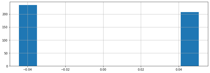
In this example, the dataset has been pre-processed such that the sex attribute takes one of two possible values (these happen to be the somewhat arbitrary numerical values 0.05068012 and -0.04464164).

2.2.4. Targets

For each patient, we may be interested in predicting a quantity of interest, the target. In our example, this is the patient’s diabetes risk.

Formally, when \((x^{(i)}, y^{(i)})\) form a training example, each \(y^{(i)} \in \mathcal{Y}\) is a target. We call \(\mathcal{Y}\) the target space.

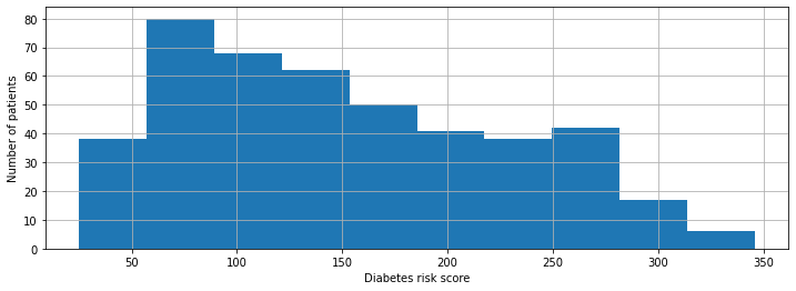
We plot our distribution of risk scores below.

plt.xlabel('Diabetes risk score')
plt.ylabel('Number of patients')
diabetes_y.hist()

<AxesSubplot:xlabel='Diabetes risk score', ylabel='Number of patients'>

Targets: Regression vs. Classification

We distinguish between two types of supervised learning problems, depending on the form of the target variable.

1. Regression: The target variable \(y\) is continuous. We are fitting a curve in a high-dimensional feature space that approximates the shape of the dataset.

2. Classification: The target variable \(y\) is discrete. Each discrete value corresponds to a class and we are looking for a hyperplane that separates the different classes.

2.2.5. The Feature Matrix

Machine learning algorithms are most easily defined using the language of linear algebra. Therefore, it will be useful to represent the entire dataset as one matrix \(X \in \mathbb{R}^{n \times d}\), of the form:

\[\begin{split} X = \begin{bmatrix} x^{(1)}_1 & x^{(2)}_1 & \ldots & x^{(n)}_1 \\ x^{(1)}_2 & x^{(2)}_2 & \ldots & x^{(n)}_2 \\ \vdots \\ x^{(1)}_d & x^{(2)}_d & \ldots & x^{(n)}_d \end{bmatrix}.\end{split}\]

Similarly, we can vectorize the target variables into a vector \(y \in \mathbb{R}^n\) of the form

\[\begin{split} y = \begin{bmatrix} y^{(1)} \\ y^{(2)} \\ \vdots \\ y^{(n)} \end{bmatrix}.\end{split}\]

2.3. Anatomy of a Supervised Learning Problem: The Learning Algorithm

Let’s now turn our attention to the second component of a supervised learning problem—the learning algorithm.

2.3.1. Three Components of a Supervised Machine Learning Algorithm

We can also define the high-level structure of a supervised learning algorithm as consisting of three components:

• A model class: the set of possible models we consider.

• An objective function, which defines how good a model is.

• An optimizer, which finds the best predictive model in the model class according to the objective function

2.3.2. The Model Class

Defining a Model

We’ll say that a model is a function

\[ f : \mathcal{X} \to \mathcal{Y} \]

that maps inputs \(x \in \mathcal{X}\) to targets \(y \in \mathcal{Y}\). Often, models have parameters \(\theta \in \Theta\) living in a set \(\Theta\). We will then write the model as

\[ f_\theta : \mathcal{X} \to \mathcal{Y} \]

to denote that it’s parametrized by \(\theta\).

Defining a Model Class

Formally, the model class is a set

\[ \mathcal{M} \subseteq \{f \mid f : \mathcal{X} \to \mathcal{Y} \}\]

of possible models that map input features to targets. When the models \(f_\theta\) are paremetrized by parameters \(\theta \in \Theta\) living in some set \(\Theta\). Thus we can also write

\[ \mathcal{M} = \{f_\theta \mid \theta \in \Theta \}.\]

An Example

One simple approach is to assume that \(x\) and \(y\) are related by a linear model of the form

\[ y=\theta_0+\theta_1 \cdot x_1+\theta_2 \cdot x_2+\ldots+\theta_d \cdot x_d \]

where \(x\) is a featurized input and \(y\) is the target. The \(\theta_j\) are the parameters of the model, \(\Theta = \mathbb{R}^{d+1}\), and \(\mathcal{M} = \{ \theta_0 + \theta_1 \cdot x_1 + \theta_2 \cdot x_2 + ... + \theta_d \cdot x_d \mid \theta \in \mathbb{R}^{d+1} \}\)

2.3.3. The Objective

Given a training set, how do we pick the parameters \(\theta\) for the model? A natural approach is to select \(\theta\) such that \(f_\theta(x^{(i)})\) is close to \(y^{(i)}\) on a training dataset \(\mathcal{D} = \{(x^{(i)}, y^{(i)}) \mid i = 1,2,...,n\}\)

Notation

To capture this intuition, we define an objective function (also called a loss function)

\[ J(f) : \mathcal{M} \to [0, \infty), \]

which describes the extent to which \(f\) “fits” the data \(\mathcal{D} = \{(x^{(i)}, y^{(i)}) \mid i = 1,2,...,n\}\).

When \(f\) is parametrized by \(\theta \in \Theta\), the objective becomes a function \(J(\theta) : \Theta \to [0, \infty).\)

Examples

What would are some possible objective functions? We will see many, but here are a few examples:

• Mean squared error:

\[ J(\theta) = \frac{1}{2n} \sum_{i=1}^n \left( f_\theta(x^{(i)}) - y^{(i)} \right)^2 \]

• Absolute (L1) error:

\[ J(\theta) = \frac{1}{n} \sum_{i=1}^n \left| f_\theta(x^{(i)}) - y^{(i)} \right| \]

These are defined for a dataset \(\mathcal{D} = \{(x^{(i)}, y^{(i)}) \mid i = 1,2,...,n\}\).

Both examples measure the difference between model predictions \(f_\theta(x^{(i)})\) and the correct targets \(y^{(i)}\). By minimizing these objectives, we are trying to find \(\theta\) such that the predictions \(\theta^\top x^{(i)}\) are as close as possible to the targets \(y^{(i)}\).

2.3.4. The Optimizer

In order to find a good model that fits the data, we also need a procedure that will actually compute the parameters \(\theta\) that minimize our learning objective (i.e., out training loss). This is the goal of the optimizer.

An optimizer takes an objective \(J\) and a model class \(\mathcal{M}\) and finds a model \(f \in \mathcal{M}\) with the smallest value of the objective \(J\).

\[ \min _{f \in \mathcal{M}} J(f) \]

When \(f\) is parametrized by \(\theta \in \Theta\), the optimizer minimizes a function \(J(\theta)\) over all \(\theta \in \Theta\).

An Example

Underneath the hood, the sklearn.linear_models.LinearRegression algorithm optimizes the MSE loss.

\[ \min _{\theta \in \mathbb{R}} \frac{1}{2 n} \sum_{i=1}^n\left(f_\theta\left(x^{(i)}\right)-y^{(i)}\right)^2 \]

We can easily measure the quality of the fit on the training set and the test set.

In the next lecture, we will learn how to minimize this objective using a clever formula. For now, let’s use sklearn to directly fit a linear model on our diabetes dataset.

# Collect 20 data points for training
diabetes_X_train = diabetes_X.iloc[-20:]
diabetes_y_train = diabetes_y.iloc[-20:]

# Create linear regression object
regr = linear_model.LinearRegression()

# Train the model using the training sets
regr.fit(diabetes_X_train, diabetes_y_train.values)

# Make predictions on the training set
diabetes_y_train_pred = regr.predict(diabetes_X_train)

# Collect 3 data points for testing
diabetes_X_test = diabetes_X.iloc[:3]
diabetes_y_test = diabetes_y.iloc[:3]

# generate predictions on the new patients
diabetes_y_test_pred = regr.predict(diabetes_X_test)

The algorithm returns a predictive model. We can visualize its predictions below.

# visualize the results
plt.xlabel('Body Mass Index (BMI)')
plt.ylabel('Diabetes Risk')
plt.scatter(diabetes_X_train.loc[:, ['bmi']], diabetes_y_train)
plt.scatter(diabetes_X_test.loc[:, ['bmi']], diabetes_y_test, color='red', marker='o')
# plt.scatter(diabetes_X_train.loc[:, ['bmi']], diabetes_y_train_pred, color='black', linewidth=1)
plt.plot(diabetes_X_test.loc[:, ['bmi']], diabetes_y_test_pred, 'x', color='red', mew=3, markersize=8)
plt.legend(['Model', 'Prediction', 'Initial patients', 'New patients'])

<matplotlib.legend.Legend at 0x12f6a46a0>

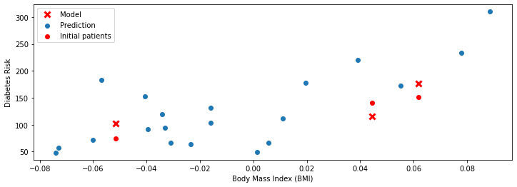
Again, the red dots are the true values of \(y\) and the red crosses are the predictions. Note that although the x-axis is still BMI, we used many additional features to make our predictions. As a result, the predictions are more accurate (the crosses are closer to the dots).

We can also confirm our intuition that the fit is good by evaluating the value of our objective.

from sklearn.metrics import mean_squared_error

print('Training set mean squared error: %.2f'
      % mean_squared_error(diabetes_y_train, diabetes_y_train_pred))
print('Test set mean squared error: %.2f'
      % mean_squared_error(diabetes_y_test, diabetes_y_test_pred))
print('Test set mean squared error on random inputs: %.2f'
      % mean_squared_error(diabetes_y_test, np.random.randn(*diabetes_y_test_pred.shape)))

Training set mean squared error: 1118.22
Test set mean squared error: 667.81
Test set mean squared error on random inputs: 15887.97

2.3.5. Summary: Components of a Supervised Machine Learning Problem

In conclusion, we defined in this lecture the task of supervised learning as well as its key elements. Formally, to apply supervised learning, we define a dataset and a learning algorithm.

\[ \underbrace{\text{Dataset}}_\text{Features, Attributes, Targets} + \underbrace{\text{Learning Algorithm}}_\text{Model Class + Objective + Optimizer } \to \text{Predictive Model} \]

A dataset consists of training examples, which are pairs of inputs and targets. Each input is a vector of features or attributes. A learning algorithm can be fully defined by a model class, objective and optimizer.

The output of a supervised learning is a predictive model that maps inputs to targets. For instance, it can predict targets on new inputs.