Lecture 5: Regularization
Contents
Lecture 5: Regularization#
This lecture starts with the question of how to evaluate supervised learning algorithms. We will identify two common failure modes of supervised learning, and develop new algorithms that address these failure modes. These algorithms will be instances of a general technique called regularization.
5.1. Two Failure Cases of Supervised Learning#
Let’s start by examining in more detail an algorithm that we introduced in an earlier lecture—polynomial regression. We will identify two settings in which this algorithm may not work well.
5.1.1. Review of Polynomial Regression#
Recall that in 1D polynomial regression, we fit a model
that is linear in \(\theta\) but non-linear in \(x\) because the features
are non-linear. Using these features, we can fit any polynomial of degree \(p\). Because the model is linear in the weights \(\theta\), we can use the normal equations to find the \(\theta\) that minimizes the mean squared error and has the best model fit. However, the resulting model can still be highly non-linear in \(x\).
5.1.1.1. Polynomials Fit the Data Well#
When we switch from linear models to polynomials, we can better fit the data and increase the accuracy of our models. This is not surprising—a polynomial is more flexible than a linear function.
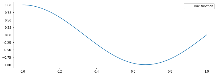
Let’s illustrate polynomial regression by implementing it on a toy dataset consisting of a cosine function.
First, we need to generate the dataset. We will do that by first defining the cosine function in numpy.
import numpy as np
np.random.seed(0)

def true_fn(X):
    return np.cos(1.5 * np.pi * X)
Let’s visualize it.
import matplotlib.pyplot as plt
plt.rcParams['figure.figsize'] = [12, 4]

X_test = np.linspace(0, 1, 100)
plt.plot(X_test, true_fn(X_test), label="True function")
plt.legend()
<matplotlib.legend.Legend at 0x120e92668>
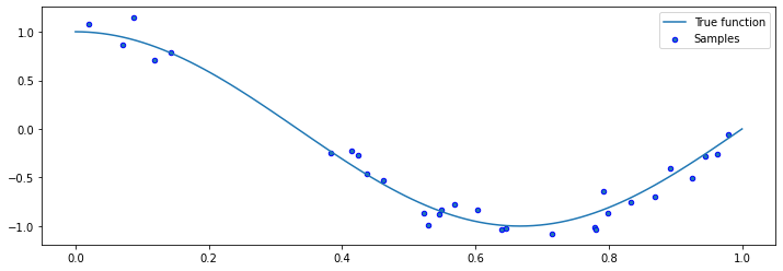
Let’s now generate datapoints around that function. We will generate random \(x\), and then generate random \(y\) using
where \(f\) is our true cosine function and \(\epsilon\) is a random noise variable.
n_samples = 30

X = np.sort(np.random.rand(n_samples))
y = true_fn(X) + np.random.randn(n_samples) * 0.1
We can visualize the samples.
plt.plot(X_test, true_fn(X_test), label="True function")
plt.scatter(X, y, edgecolor='b', s=20, label="Samples")
plt.legend()
<matplotlib.legend.Legend at 0x12111c860>
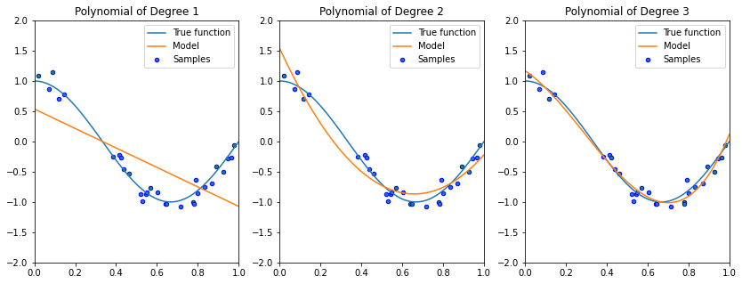
These samples represent our dataset. We can now try to fit it using a number of different models, including linear functions and polynomials of various degrees.
Although fitting a linear model does not work well, quadratic or cubic polynomials improve the fit.
degrees = [1, 2, 3]
plt.figure(figsize=(14, 5))
for i in range(len(degrees)):
    ax = plt.subplot(1, len(degrees), i + 1)

    polynomial_features = PolynomialFeatures(degree=degrees[i], include_bias=False)
    linear_regression = LinearRegression()
    pipeline = Pipeline([("pf", polynomial_features), ("lr", linear_regression)])
    pipeline.fit(X[:, np.newaxis], y)

    ax.plot(X_test, true_fn(X_test), label="True function")
    ax.plot(X_test, pipeline.predict(X_test[:, np.newaxis]), label="Model")
    ax.scatter(X, y, edgecolor='b', s=20, label="Samples")
    ax.set_xlim((0, 1))
    ax.set_ylim((-2, 2))
    ax.legend(loc="best")
    ax.set_title("Polynomial of Degree {}".format(degrees[i]))
5.1.1.2. Towards Higher-Degree Polynomial Features?#
As we increase the complexity of our model class \(\mathcal{M}\) to include even higher degree polynomials, we are able to fit the data even better.
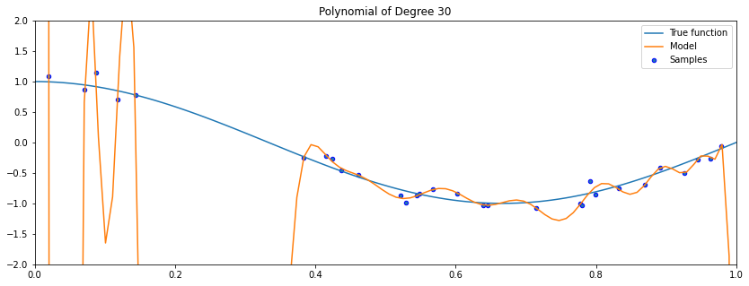
What happens if we further increase the degree of the polynomial?
degrees = [30]
plt.figure(figsize=(14, 5))
for i in range(len(degrees)):
    ax = plt.subplot(1, len(degrees), i + 1)

    polynomial_features = PolynomialFeatures(degree=degrees[i], include_bias=False)
    linear_regression = LinearRegression()
    pipeline = Pipeline([("pf", polynomial_features), ("lr", linear_regression)])
    pipeline.fit(X[:, np.newaxis], y)

    X_test = np.linspace(0, 1, 100)
    ax.plot(X_test, true_fn(X_test), label="True function")
    ax.plot(X_test, pipeline.predict(X_test[:, np.newaxis]), label="Model")
    ax.scatter(X, y, edgecolor='b', s=20, label="Samples")
    ax.set_xlim((0, 1))
    ax.set_ylim((-2, 2))
    ax.legend(loc="best")
    ax.set_title("Polynomial of Degree {}".format(degrees[i]))

As the degree of the polynomial increases to the size of the dataset, we are increasingly able to fit every point in the dataset.
However, this results in a highly irregular curve: its behavior outside the training set is wildly inaccurate!
5.1.2. Overfitting and Underfitting#
We have seen above a clear failure of polynomial regression. In fact, this failure represents an example of a more general phenomenon that we call overfitting. Overfitting—and its opposite, underfitting—represent the most important failure modes of all supervised learning algorithms.
5.1.2.1. Definitions#
Overfitting#
Overfitting is one of the most common failure modes of machine learning.
A very expressive model (e.g., a high degree polynomial) fits the training dataset perfectly.
But the model makes highly incorrect predictions outside this dataset, and doesn’t generalize.
In other words, if the model is too expressive (like a high degree polynomial), we are going to fit the training dataset perfectly; however, the model will make incorrect predictions at points right outside this dataset, and will also not generalize well to unseen data.
Underfitting#
A related failure mode is underfitting.
A small model (e.g. a straight line), will not fit the training data well.
Therefore, it will also not be accurate on new data.
If the model is too small (like the linear model in the above example), it will not generalize well to unseen data because it is not sufficiently complex to fit the true structure of the dataset.
Finding the tradeoff between overfitting and underfitting is one of the main challenges in applying machine learning.
5.1.2.2. Overfitting vs. Underfitting: Evaluation#
We can diagnose overfitting and underfitting by measuring performance on a separate held out dataset (not used for training).
If training performance is high but holdout performance is low, we are overfitting.
If training performance is low but holdout performance is low, we are underfitting.
Let’s look at this via an example. Below, we are generating a separate held out dataset from the same data generating process (represented via red dots on the figures). We fit three different models (the orange curves) to our training set (the blue dots), and observe their performance.
degrees = [1, 20, 5]
titles = ['Underfitting', 'Overfitting', 'A Good Fit']
plt.figure(figsize=(14, 5))
for i in range(len(degrees)):
    ax = plt.subplot(1, len(degrees), i + 1)

    polynomial_features = PolynomialFeatures(degree=degrees[i], include_bias=False)
    linear_regression = LinearRegression()
    pipeline = Pipeline([("pf", polynomial_features), ("lr", linear_regression)])
    pipeline.fit(X[:, np.newaxis], y)

    ax.plot(X_test, true_fn(X_test), label="True function")
    ax.plot(X_test, pipeline.predict(X_test[:, np.newaxis]), label="Model")
    ax.scatter(X, y, edgecolor='b', s=20, label="Samples", alpha=0.2)
    ax.scatter(X_holdout[::3], y_holdout[::3], edgecolor='r', s=20, label="Samples")
    ax.set_xlim((0, 1))
    ax.set_ylim((-2, 2))
    ax.legend(loc="best")
    ax.set_title("{} (Degree {})".format(titles[i], degrees[i]))
    ax.text(0.05,-1.7, 'Holdout MSE: %.4f' % ((y_holdout-pipeline.predict(X_holdout[:, np.newaxis]))**2).mean())
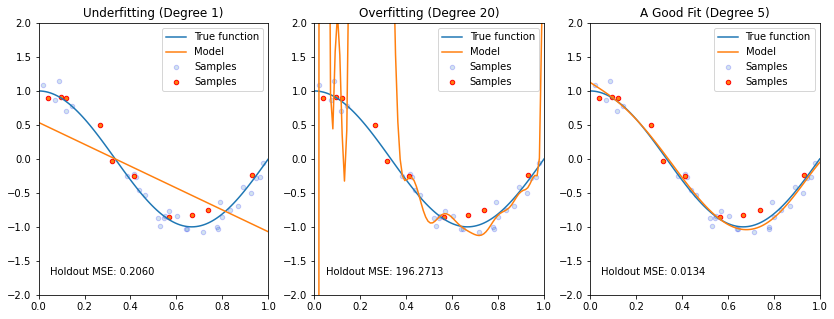
In the above example, the linear model is clearly too simple to fit the cosine function. It has an MSE of 0.2060 on the red held-out set. The middle model is clearly overfitting and gets a massive MSE on the red dots. The right-most figure is clearly the best fit, and it gets the lowest MSE by far.
Thus, we can detect overfitting and underfitting quantitatively by measuring performance on held out data. We will come back to this later.
5.1.2.3. How to Fix Overfitting and Underfitting#
What if a model doesn’t fit the training set well? We may try the following:
Create richer features that will make the dataset easier to fit.
Use a more expressive model family (neural nets vs. linear models). A more expressive model is more likely to fit the data well.
Try a better optimization procedure. Sometimes the fit is bad simply because we haven’t trained our model sufficiently well.
We will also see many ways of dealing with overfitting, but here are some ideas:
Use a simpler model family (linear models vs. neural nets)
Keep the same model, but collect more training data. Given a model family, it will be difficult to find a highly fitting model if the dataset is very large.
Modify the training process to penalize overly complex models. We will come back to this last point in a lot more detail.
5.2. Evaluating Supervised Learning Models#
We have just seen that supervised learning algorithms can fail in practice. In particular they have two clear failure modes—overfitting and underfitting. In order to avoid these failures, the first step is to understand how to evaluate supervised models in a principled way.
5.2.1. What Is A Good Supervised Learning Model?#
Our previous example involving polynomial regression should strongly suggests the following principle for determining whether a supervised model is good or not. A good supervised model is one that makes accurate predictions on new data that it has not seen at training time.
What does it mean to make accurate predictions? Here are a few examples:
Accurate predictions of diabetes risk on patients
Accurate object detection in new scenes
Correct translation of new sentences
Note, however, that other types of definitions of good performance exist from the ones above. For example, we may be interested in whether the model discovers useful structure in the data. This is different from simply asking for good predictive accuracy. We will come back to other performance criteria later in the course.
5.2.1.1. When Do We Get Good Performance on New Data?#
We need to make formal the notion of being accurate on new data. For this we will introduce notation for a holdout dataset, which is a second supervised learning dataset consisting of \(m\) training instances.
Crucially, this dataset is distinct from the training dataset \(\mathcal{D}\).
Let’s say we have trained a model on \(\mathcal{D}\); when will it be accurate on \(\dot{\mathcal{D}}\)? Or, more concretely, suppose you have a classification model trained on images of cats and dogs. On which dataset will it perform better?
A dataset of German shepherds and siamese cats?
A dataset of birds and reptiles?
Clearly it will be more accurate on the former. Intuitively, ML are accurate on new data, if it is similar to the training data.
5.2.2 Data Distribution#
We are now going to make the above intuition more precise via a new concept that is very important in machine learning—the data distribution.
It is standard in machine learning to assume that data is sampled from some probability distribution \(P_\text{data}\), which we call the data distribution. We will denote this as
The training set \(\mathcal{D} = \{(x^{(i)}, y^{(i)}) \mid i = 1,2,...,n\}\) consists of independent and identically distributed (IID) samples from \(\mathbb{P}\).
5.2.2.1. IID Sampling#
The key assumption is that the training examples are independent and identically distributed (IID).
Each training example is from the same distribution.
This distribution doesn’t depend on previous training examples.
Example: Flipping a coin. Each flip has same probability of heads & tails and doesn’t depend on previous flips.
Counter-Example: Yearly census data. The population in each year will be close to that of the previous year.
5.2.2.2. Motivation#
Why assume that the dataset is sampled from a distribution?
The process we model may be effectively random. If \(y\) is a stock price, there is randomness in the market that cannot be captured by a deterministic model.
There may be noise and randomness in the data collection process itself (e.g., collecting readings from an imperfect thermometer).
We can use probability and statistics to analyze supervised learning algorithms and prove that they work. The key idea is that if we train a model on data sampled from \(P_\text{data}\), it will also be accurate on new (previously unseen) data that is also sampled from \(P_\text{data}\).
5.2.2.3. An Example#
Let’s implement an example of a data distribution in numpy. Below, we are defining the same cosine function that we have previously seen.
import numpy as np
np.random.seed(0)

def true_fn(X):
    return np.cos(1.5 * np.pi * X)
Let’s visualize it.
import matplotlib.pyplot as plt
plt.rcParams['figure.figsize'] = [12, 4]

X_test = np.linspace(0, 1, 100)
plt.plot(X_test, true_fn(X_test), label="True function")
plt.legend()
<matplotlib.legend.Legend at 0x120e92668>

Let’s now draw samples from the distribution. We will generate random \(x\), and then generate random \(y\) using
for a random noise variable \(\epsilon\).
n_samples = 30

X = np.sort(np.random.rand(n_samples))
y = true_fn(X) + np.random.randn(n_samples) * 0.1
We visualize the samples below.
plt.plot(X_test, true_fn(X_test), label="True function")
plt.scatter(X, y, edgecolor='b', s=20, label="Samples")
plt.legend()
<matplotlib.legend.Legend at 0x12111c860>

Let’s also genenerate a holdout dataset.
n_samples, n_holdout_samples = 30, 30

X = np.sort(np.random.rand(n_samples))
y = true_fn(X) + np.random.randn(n_samples) * 0.1
X_holdout = np.sort(np.random.rand(n_holdout_samples))
y_holdout = true_fn(X_holdout) + np.random.randn(n_holdout_samples) * 0.1

plt.plot(X_test, true_fn(X_test), label="True function")
plt.scatter(X, y, edgecolor='b', s=20, label="Samples")
plt.scatter(X_holdout, y_holdout, edgecolor='r', s=20, label="Holdout Samples")
plt.legend()
<matplotlib.legend.Legend at 0x121440f28>
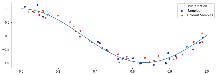
We now have defined two supervised learning datasets: a training set \(\mathcal{D}\) (in blue), and a separate hold out set \(\dot{\mathcal{D}}\) (in red). If we train a supervised model on \(\mathcal{D}\) (in a way that avoids overfitting and underfitting), this model will be accurate on \(\dot{\mathcal{D}}\) (and in fact, on any hold out dataset sampled from the same data distribution \(P_\text{data}\) that generated \(\mathcal{D}\).
5.2.3. Performance on a Holdout Set#
Formally, we consider a supervised model \(f_\theta\) to be a “good” model (i.e., an accurate model) if it performs well on a holdout set \(\dot{\mathcal{D}}\) according to some metric
Here, \(L : \mathcal{X}\times\mathcal{Y} \to \mathbb{R}\) is a performance metric or a loss function that we get to choose.
The choice of the performance metric \(L\) depends on the specific problem and our goals:
\(L\) can be the training objective: mean squared error, cross-entropy
In classification, \(L\) is often just accuracy: is \(\dot y^{(i)} = f_\theta(\dot x^{(i)})\)?
\(L\) can also implement a task-specific metric: \(R^2\) metric (see Homework 1) for regression, precision/recall score for document retrieval, etc.
For example, in a classification setting, we may be interested in the accuracy of the model. Thus, we want the % of misclassified inputs
to be small.
Here \(\mathbb{I}\left( A \right)\) is an indicator function that equals one if \(A\) is true and zero otherwise.
The key thing to note is that for large enough holdout sets \(\dot{\mathcal{D}}\), our estimate of performance on \(\dot{\mathcal{D}}\) we will be an accurate estimate of performance on new datapoints sampled from the data distribution \(P_\text{data}\).
5.3. A Framework for Applying Supervised Learning#
In practice, we use not one but multiple holdout sets when developing machine learning models. These multiple datasets are part of an interactive framework for developing ML algorithms that we will describe next.
5.3.1. Datasets for Model Development#
When developing machine learning models, it is customary to work with three datasets:
Training set: Data on which we train our algorithms.
Development set (validation or holdout set): Data used for tuning algorithms.
Test set: Data used to evaluate the final performance of the model.
The test set is best thought of as a small amount of data that is put aside and never used during model development—we only use it to evaluate our final model. This is to ensure an unbiased estimate of performance for the final model.
The development set on the other hand is constantly used for tasks such as hyperparameter selection (more on that later).
When beginning a new project (e.g., a Kaggle competition), it is common to split all the available data into the above three datasets. A common splitting ratio is approximately 70%, 15%, 15%. However, we will see later some improved splitting strategies as well.
5.3.2. Model Development Workflow#
The typical way in which these datasets are used is:
Training: Try a new model and fit it on the training set.
Model Selection: Estimate performance on the development set using metrics. Based on results, try a new model idea in step #1.
Evaluation: Finally, estimate real-world performance on test set.
When we start developing a new supervised learning model we often only have a rough guess as to what a good model looks like. We start with this initial guess—this includes a choice of model family, features, hyperparameters, etc.—and we train it.
We then evaluate this model on the development set and adjust our initial guess. For example, if we see that our initial model is overfitting, we that know we need to make it smaller. After several iteration of this process, we will fix many of the problems observed on the development set.
Once we are satisfied with development set performance, we evaluate the model on the test set. This represents our final unbiased estimate of performance before we release the model into the world.
5.3.2.1 Choosing Validation and Test Sets#
How should one choose the development and test sets? We highlight two important considerations.
Distributional Consistency: The development and test sets should be from the data distribution that we will see at deployment time.
Dataset Size: The development and test sets should be large enough to estimate future performance. On small datasets, about 30% of the data can be used for development and testing. On larger datasets, it usually not useful to reserve more than a few thousand instances—these are enough to ensure small error bars on our performance estimates.
5.4. L2 Regularization#
Thus far, we have identified two common failure modes of supervised learning algorithms (overfitting and underfitting), and we have discussed how to evaluate models and detect these failure modes.
Let’s now look at a technique that helps avoid overfitting altogether.
5.4.0. Review: Overfitting#
Recall that overfitting is one of the most common failure modes of machine learning.
A very expressive model (a high degree polynomial) fits the training dataset perfectly.
The model also makes wildly incorrect prediction outside this dataset, and doesn’t generalize.
We can visualize overfitting by trying to fit a small dataset with a high degree polynomial.
degrees = [30]
plt.figure(figsize=(14, 5))
for i in range(len(degrees)):
    ax = plt.subplot(1, len(degrees), i + 1)

    polynomial_features = PolynomialFeatures(degree=degrees[i], include_bias=False)
    linear_regression = LinearRegression()
    pipeline = Pipeline([("pf", polynomial_features), ("lr", linear_regression)])
    pipeline.fit(X[:, np.newaxis], y)

    X_test = np.linspace(0, 1, 100)
    ax.plot(X_test, true_fn(X_test), label="True function")
    ax.plot(X_test, pipeline.predict(X_test[:, np.newaxis]), label="Model")
    ax.scatter(X, y, edgecolor='b', s=20, label="Samples")
    ax.set_xlim((0, 1))
    ax.set_ylim((-2, 2))
    ax.legend(loc="best")
    ax.set_title("Polynomial of Degree {}".format(degrees[i]))
In this example, the polynomial passes through every training set points, but its fit is very bad outside the small training set.
5.4.1. Regularization#
Recall that we talked about a few ways of mitigating overfitting—making the model smaller, giving it more data, and modifying the training process to avoid the selection of models that overfit. Regularization is a technique that takes the latter strategy.
Intuitively, the idea of regularization is to penalize complex models that may overfit the data. In the previous example, a less complex would rely less on polynomial terms of high degree.
5.4.1.1. Definition#
More formally, the idea of regularization is to train models with an augmented objective \(J : \mathcal{M} \to \mathbb{R}\) defined over a training dataset \(\mathcal{D}\) of size \(n\) as
Let’s examine this objective. It features three important components:
A loss function \(L(y, f(x))\) such as the mean squared error. This is usually a standard supervised learning loss.
A regularizer \(R : \mathcal{M} \to \mathbb{R}\) that penalizes models that are overly complex. Specifically, this term takes in a function and outputs a large score for models that it considers being overly complex.
A regularization parameter \(\lambda > 0\), which controls the strength of the regularizer.
When the model \(f_\theta\) is parametrized by parameters \(\theta\), we also use the following notation:
Next, let’s see some examples of what a regularizer could look like.
5.4.2. L2 Regularization#
How can we define a regularizer \(R: \mathcal{M} \to \mathbb{R}\) to control the complexity of a model \(f \in \mathcal{M}\)? In the context of linear models \(f_\theta(x) = \theta^\top x\), a widely used approach is called L2 regularization.
5.4.2.1. Definition#
L2 regularization defines the following objective:
Let’s examine the components of this objective.
Note that the regularizer \(R : \Theta \to \mathbb{R}\) is the function \(R(\theta) = ||\theta||_2^2 = \sum_{j=1}^d \theta_j^2.\) This is also known as the L2 norm of \(\theta\).
The regularizer penalizes large parameters. This prevents us from relying on any single feature and penalizes very irregular solutions. It is an empirical fact that models that tend to overfit (like the polynomials in our examples) tend to have weights with a very large L2 norm. By penalizing this norm, we are penalizing complex models.
Finally, note that although we just defined L2 regularization in the context of linear regression, any model that has parameters can be regularized by adding to the objective the L2 norm of these parameters. Thus, the technique can be used with logistic regression, neural networks, and many other models.
5.4.2.2. L2 Regularization for Polynomial Regression#
Let’s consider an application to the polynomial model we have seen so far. Given polynomial features \(\phi(x)\), we optimize the following objective:
We implement regularized and polynomial regression of degree 15 on three random training sets sampled from the same distribution.
from sklearn.linear_model import Ridge

degrees = [15, 15, 15]
plt.figure(figsize=(14, 5))
for idx, i in enumerate(range(len(degrees))):
    # sample a dataset
    np.random.seed(idx)
    n_samples = 30
    X = np.sort(np.random.rand(n_samples))
    y = true_fn(X) + np.random.randn(n_samples) * 0.1

    # fit a least squares model
    polynomial_features = PolynomialFeatures(degree=degrees[i], include_bias=False)
    linear_regression = LinearRegression()
    pipeline = Pipeline([("pf", polynomial_features), ("lr", linear_regression)])
    pipeline.fit(X[:, np.newaxis], y)

    # fit a Ridge model
    polynomial_features = PolynomialFeatures(degree=degrees[i], include_bias=False)
    linear_regression = Ridge(alpha=0.1) # sklearn uses alpha instead of lambda
    pipeline2 = Pipeline([("pf", polynomial_features), ("lr", linear_regression)])
    pipeline2.fit(X[:, np.newaxis], y)

    # visualize results
    ax = plt.subplot(1, len(degrees), i + 1)
    # ax.plot(X_test, true_fn(X_test), label="True function")
    ax.plot(X_test, pipeline.predict(X_test[:, np.newaxis]), label="No Regularization")
    ax.plot(X_test, pipeline2.predict(X_test[:, np.newaxis]), label="L2 Regularization")
    ax.scatter(X, y, edgecolor='b', s=20, label="Samples")
    ax.set_xlim((0, 1))
    ax.set_ylim((-2, 2))
    ax.legend(loc="best")
    ax.set_title("Dataset sample #{}".format(idx))
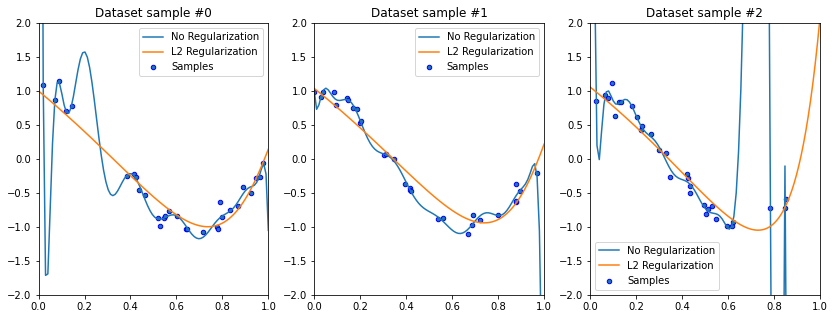
It’s an empirical fact that in order to define a very irregular function, we need very large polynomial weights.
Forcing the model to use small weights prevents it from learning irregular functions.
print('Non-regularized weights of the polynomial model need to be large to fit every point:')
print(pipeline.named_steps['lr'].coef_[:4])
print()

print('By regularizing the weights to be small, we force the curve to be more regular:')
print(pipeline2.named_steps['lr'].coef_[:4])
Non-regularized weights of the polynomial model need to be large to fit every point:
[-3.02370887e+03  1.16528860e+05 -2.44724185e+06  3.20288837e+07]

By regularizing the weights to be small, we force the curve to be more regular:
[-2.70114811 -1.20575056 -0.09210716  0.44301292]
In the above example, the weights of the best-fit degree 15 polynomial are huge: they are on the order of \(10^3\) to \(10^7\). By regularizing the model, we are forcing the weights to be small—less than \(10^0\) in this example, As expected, a polynomial with small weights cannot reproduce the highly “wiggly” shape of the overfitting polynomial, and thus does not suffer from the same failure mode.
5.4.2.3. How to Choose \(\lambda\)? Hyperparameter Search#
Note that regularization has introduced a new parameter into our model—the regularization strength \(\lambda\).
We refer to \(\lambda\) as a hyperparameter, because it’s a parameter that controls other parameters and is not selected via the learning algorithm. Higher values of \(\lambda\) induce a small norm for \(\theta\).
Note that we do not want to learn \(\lambda\) from data like regular parameters—if we did, the optimizer would just set it to zero to get the best possible training fit.
How do we choose \(\lambda\) then? We select the \(\lambda\) that yields the best model performance on the development set. Thus, we are in a sense choosing \(\lambda\) by minimizing the training loss on the development set. Over time this can lead us to overfit the development set; however, there is usually only a very small number of hyperparameters, and the problem is not as pronounced as regular overfitting.
5.4.3. Normal Equations for L2-Regularized Linear Models#
How, do we fit regularized models? As in the linear case, we can do this easily by deriving generalized normal equations!
Let \(L(\theta) = \frac{1}{2} (X \theta - y)^\top (X \theta - y)\) be our least squares objective. We can write the L2-regularized objective as:
This allows us to derive the gradient as follows:
We used the derivation of the normal equations for least squares to obtain \(\nabla_\theta L(\theta)\) as well as the fact that: \(\nabla_x x^\top x = 2 x\).
We can set the gradient to zero to obtain normal equations for the Ridge model:
Hence, the value \(\theta^*\) that minimizes this objective is given by:
Note that the matrix \((X^\top X + \lambda I)\) is always invertible, which addresses a problem with least squares that we saw earlier.
5.4.4. Algorithm: Ridge Regression#
These derivations yield a new algorithm, which is known as L2-regularized ordinary least squares or simply Ridge regression.
Type: Supervised learning (regression)
Model family: Linear models
Objective function: L2-regularized mean squared error
Optimizer: Normal equations
Ridge regression can be used to fit models with highly non-linear features (like high-dimensional polynomial regression), while keeping overfitting under control.
5.5. L1 Regularization and Sparsity#
The L2 norm is not the only type of regularizer that can be used to mitigate overfitting. We will now look at another approach called L1 regularization, which will have an important new property called sparsity.
5.5.1. L1 Regularization#
5.5.1.1. Definition#
Another closely related approach to L2 regularization is to penalize the size of the weights using the L1 norm.
In the context of linear models \(f(x) = \theta^\top x\), L1 regularization yields the following objective:
Let’s examine the components of this objective.
As before, the objective contains a supervised loss \(L\) and a hyper-parameter \(\lambda\).
The regularizer \(R : \mathcal{M} \to \mathbb{R}\) is now \(R(\theta) = ||\theta||_1 = \sum_{j=1}^d |\theta_j|.\) This is known as the L1 norm of \(\theta\).
This regularizer also penalizes large weights. However, it additionally forces most weights to decay to zero, as opposed to just being small.
5.5.1.2. Algorithm: Lasso#
L1-regularized linear regression is also known as the Lasso (least absolute shrinkage and selection operator).
Type: Supervised learning (regression)
Model family: Linear models
Objective function: L1-regularized mean squared error
Optimizer: gradient descent, coordinate descent, least angle regression (LARS) and others
Unlike Ridge regression, the Lasso does not have an analytical formula for the best-fit parameters. In practice, we resort to iterative numerical algorithms, including variations of gradient descent and more specialized procedures.
5.5.2. Sparsity#
Like L2 regularization, the L1 approach makes model weights small. However, it doesn’t just make the weights small—it sets some of them exactly zero. This property of the weights is called sparsity, and can be very useful in practice.
5.5.2.1. Definition#
More formally, a vector is said to be sparse if a large fraction of its entires is zero. Thus, L1-regularized linear regression produces sparse parameters \(\theta\).
Why is sparsity useful?
It makes the model more interpretable. If we have a large number of features, the Lasso will set most of their parameters zero, thus effectively excluding them. This allows us to focus our attention on a small number of relevant features.
Sparsity can also make models computationally more tractable. Once the model has set certain weights to zero—we can ignore their corresponding features entirely. This avoids us from spending and computation or memory on these features.
5.5.2.2. Visualizing Weights in Ridge and Lasso#
To better understand sparsity, we fit Ridge and Lasso on the UCI diabetes dataset and observe the magnitude of each weight (colored lines) as a function of the regularization parameter.
Below is Ridge—each colored line represents the magnitude of each of the ten different model parameters as a function of regularization strength. Clearly, the weights become smaller as we regularize more.
# based on https://scikit-learn.org/stable/auto_examples/linear_model/plot_ridge_path.html
from sklearn.datasets import load_diabetes
from sklearn.linear_model import Ridge
from matplotlib import pyplot as plt

X, y = load_diabetes(return_X_y=True)

# create ridge coefficients
alphas = np.logspace(-5, 2,  )
ridge_coefs = []
for a in alphas:
    ridge = Ridge(alpha=a, fit_intercept=False)
    ridge.fit(X, y)
    ridge_coefs.append(ridge.coef_)

# plot ridge coefficients
plt.figure(figsize=(14, 5))
plt.plot(alphas, ridge_coefs)
plt.xscale('log')
plt.xlabel('Regularization parameter (lambda)')
plt.ylabel('Magnitude of model parameters')
plt.title('Ridge coefficients as a function of the regularization')
plt.axis('tight')
(4.466835921509635e-06,
 223.872113856834,
 -868.4051623855127,
 828.0533448059361)
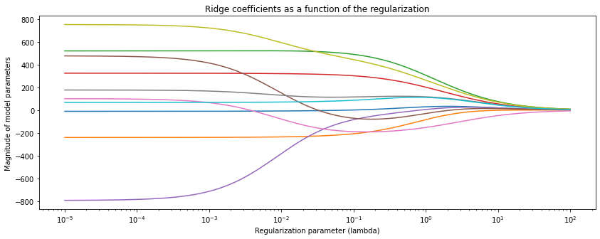
However, the Ridge model does not produce sparse weights—the weights are never exactly zero. Let’s now compare it to a Lasso model.
# Based on: https://scikit-learn.org/stable/auto_examples/linear_model/plot_lasso_lars.html
import warnings
warnings.filterwarnings("ignore")
from sklearn.datasets import load_diabetes
from sklearn.linear_model import lars_path

# create lasso coefficients
X, y = load_diabetes(return_X_y=True)
_, _, lasso_coefs = lars_path(X, y, method='lasso')
xx = np.sum(np.abs(lasso_coefs.T), axis=1)

# plot ridge coefficients
plt.figure(figsize=(14, 5))
plt.subplot('121')
plt.plot(alphas, ridge_coefs)
plt.xscale('log')
plt.xlabel('Regularization Strength (lambda)')
plt.ylabel('Magnitude of model parameters')
plt.title('Ridge coefficients as a function of regularization strength $\lambda$')
plt.axis('tight')

# plot lasso coefficients
plt.subplot('122')
plt.plot(3500-xx, lasso_coefs.T)
ymin, ymax = plt.ylim()
plt.ylabel('Magnitude of model parameters')
plt.xlabel('Regularization Strength (lambda)')
plt.title('LASSO coefficients as a function of regularization strength $\lambda$')
plt.axis('tight')
(-133.00520290292727, 3673.000247757282, -869.357335763701, 828.4524952229654)
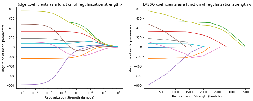
Observe how the Lasso parameters become progressively smaller, until they reach exactly zero, and then they stay at zero.
5.5.3. Why Does L1 Regularization Produce Sparsity?#
We conclude with some intuition for why L1 regularization induces sparsity. This is a more advanced topic that is not essential for understanding the most important ideas in this section.
5.5.3.1. Regularizing via Constraints#
Consider a regularized problem with a penalty term:
Alternatively, we may enforce an explicit constraint on the complexity of the model:
We will not prove this, but solving this problem is equivalent to solving the penalized problem for some \(\lambda > 0\) that’s different from \(\lambda'\). In other words,
We can regularize by explicitly enforcing \(R(\theta)\) to be less than a value instead of penalizing it.
For each value of \(\lambda\), we are implicitly setting a constraint of \(R(\theta)\).
An Example#
This is what constraint-based regularization looks like for the linear models we have seen thus far:
where \(||\cdot||\) can either be the L1 or L2 norm.
5.5.3.2. Sparsity in L1 vs. L2 Regularization#
The following image by Divakar Kapil and Hastie et al. explains the difference between the two norms.
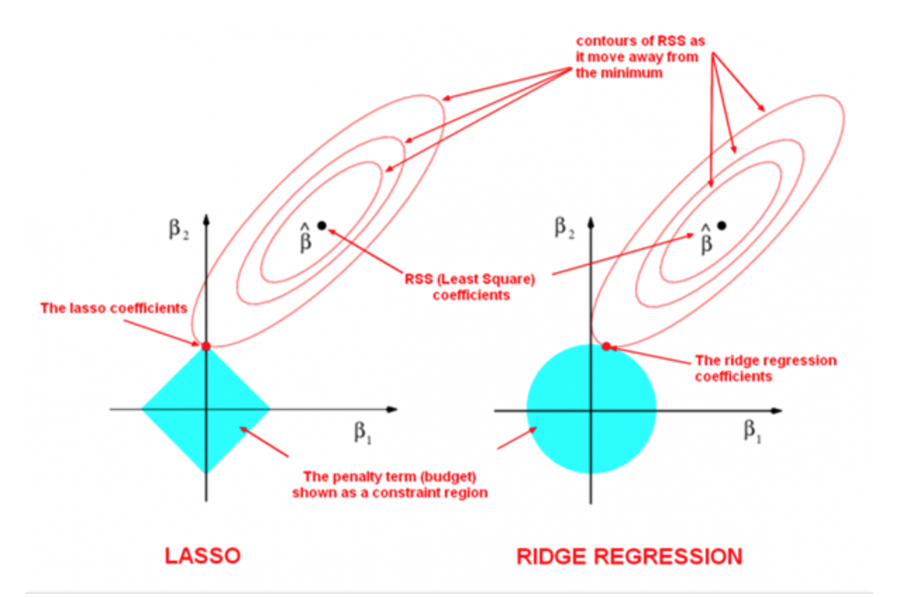
The ellipses represent the level curves of the mean squared error (MSE) loss function used by both Ridge and Lasso. The unregularized minimizer is indicated by a black dot (\(\hat\beta\)).
However, the loss is regularized, and the parameters are constrained to live in the light blue regions. These are the L1 ball around zero (on the left) and the L2 ball around zero (on the right). Therefore, the parameters chosen by both models are point with the smallest MSE loss that are within the light blue feasible region.
In order to find these points, we have to find the level curve that is tangent to the feasible region (this is shown in the figure). On the right hand side, the shape of the L2 feasible region is round and it’s unlikely that the tanget point will be one that is sparse.
However, in the L1 case, the level curve will most likely be tangent to the L1 feasible region at a “vertex” of the diamond. These “vertices” are aligned with the axes—therefore at these points some of the coefficients are exactly zero. This is the intuition for why L1 produces sparse parameter vectors.
5.6. Why Does Supervised Learning Work?#
We have started this lecture with an example of when supervised learning doesn’t work. Let’s conclude it with a more detailed argument explaining when and why supervised learning does work.
This advanced material is not essential to understand the rest of the lecture.
First, let’s begin by recalling again our intuitive definition of supervised learning.
First, we collect a dataset of labeled training examples.
We train a model to output accurate predictions on this dataset.
We have seen that a good predictive model is one that makes accurate predictions on new data that it has not seen at training time. We will now prove that under some conditions and given enough data is guaranteed to be accurate on enw data coming from the same data distribution.
5.6.1. Some Assumptions and Definitions#
5.6.1.1. Data Distribution#
We will assume that data is sampled from a probability distribution \(\mathbb{P}\), which we will call the data distribution. We will denote this as
The training set \(\mathcal{D} = \{(x^{(i)}, y^{(i)}) \mid i = 1,2,...,n\}\) consists of independent and identicaly distributed (IID) samples from \(\mathbb{P}\).
5.6.1.2. Holdout Dataset#
A holdout dataset
is sampled IID from the same distribution \(\mathbb{P}\), and is distinct from the training dataset \(\mathcal{D}\).
5.6.1.2. Evaluating Performance on a Holdout Set#
Intuitively, a supervised model \(f_\theta\) is successful if it performs well on a holdout set \(\dot{\mathcal{D}}\) according to some measure
Here, \(L : \mathcal{X}\times\mathcal{Y} \to \mathbb{R}\) is a performance metric or a loss function that we get to choose.
The choice of the performance metric \(L\) depends on the specific problem and our goals. For example, in a classification setting, we may be interested in the accuracy of the model. Thus, we want the % of misclassified inputs
to be small. Here \(\mathbb{I}\left( A \right)\) is an indicator function that equals one if \(A\) is true and zero otherwise.
5.6.2. Performance on Out-of-Distribution Data#
Intuitively, a supervised model \(f_\theta\) is successful if it performs well in expectation on new data \(\dot x, \dot y\) sampled from the data distribution \(\mathbb{P}\):
Here, \(L : \mathcal{X}\times\mathcal{Y} \to \mathbb{R}\) is a performance metric and we take its expectation or average over all the possible samples \(\dot x, \dot y\) from \(\mathbb{P}\).
Recall that formally, an expectation \(\mathbb{E}_{x)\sim {P}} f(x)\) is \(\sum_{x \in \mathcal{X}} f(x) P(x)\) if \(x\) is discrete and \(\int_{x \in \mathcal{X}} f(x) P(x) dx\) if \(x\) is continuous. Intuitively,
is the performance on an infinite-sized holdout set, where we have sampled every possible point.
In practice, we cannot measure
on infinite data. We approximate its performance with a sample \(\dot{\mathcal{D}}\) from \(\mathbb{P}\) and we measure
If the number of IID samples \(m\) is large, this approximation holds (we call this a Monte Carlo approximation).
For example, in a classification setting, we may be interested in the accuracy of the model. We want a small probability of making an error on a new \(\dot x, \dot y \sim \mathbb{P}\):
We approximate this via the % of misclassifications on \(\dot{\mathcal{D}}\) sampled from \(\mathbb{P}\):
Here, \(\mathbb{I}\left( A \right)\) is an indicator function that equals one if \(A\) is true and zero otherwise.
To summarize, a supervised model \(f_\theta\) performs well when
Under which conditions is supervised learning guaranteed to give us a good model?
5.6.3. Machine Learning Provably Works#
Suppose that we choose \(f \in \mathcal{M}\) on a dataset \(\mathcal{D}\) of size \(n\) sampled IID from \(\mathbb{P}\) by minimizing
Let \(f^*\), the best model in \(\mathcal{M}\):
Then, as \(n \to \infty\), the performance of \(f\) approaches that of \(f^*\).
5.6.3.1. Short Proof of Why Machine Learning Works#
We say that a classification model \(f\) is accurate if its probability of making an error on a new random datapoint is small:
for \(\dot{x}, \dot{y} \sim \mathbb{P}\), for some small \(\epsilon > 0\) and some definition of accuracy.
We can also say that the model \(f\) is inaccurate if it’s probability of making an error on a random holdout sample is large:
or equivalently
In order to prove that supervised learning works, we will make two simplifying assumptions:
We define a model class \(\mathcal{M}\) containing \(H\) different models
One of these models fits the training data perfectly (is accurate on every point) and we choose that model.
(Both of these assumptions can be relaxed.)
Claim: The probability that supervised learning will return an inaccurate model decreases exponentially with training set size \(n\).
A model \(f\) is inaccurate if \(\mathbb{P} \left[ \dot y= f(\dot x) \right] \leq 1-\epsilon\). The probability that an inaccurate model \(f\) perfectly fits the training set is at most \(\prod_{i=1}^n \mathbb{P} \left[ \dot y= f(\dot x) \right] \leq (1-\epsilon)^n\).
We have \(H\) models in \(\mathcal{M}\), and any of them could be in accurate. The probability that at least one of at most \(H\) inaccurate models willl fit the training set perfectly is \(\leq H (1-\epsilon)^n\).
Therefore, the claim holds.