Lecture 14: Kernels#

In this lecture, we will introduce a new and important concept in machine learning: the kernel. So far, the majority of the machine learning models we have seen have been linear. Kernels are a general way to make many of these models non-linear.

14.1. The Kernel Trick in SVMs#

In the previous two lectures, we introduced linear SVMs. Kernels will be a way to make the SVM algorithm suitable for dealing with non-linear data.

14.1.1. Review: Support Vector Machines.#

We are given a training dataset $\mathcal{D} = \{(x^{(1)}, y^{(1)}), (x^{(2)}, y^{(2)}), \ldots, (x^{(n)}, y^{(n)})\}$. We are interested in binary classification, in which the target variable $y$ is discrete and takes on one of $K=2$ possible values. In this lecture, we assume that $\mathcal{Y} = \{-1, +1\}$.

Linear models for this binary classification can take the form

\[ \begin{align*} f_\theta(x) = \theta^\top \phi(x) + \theta_0, \end{align*} \]

where $x$ is the input and $y \in \{-1, 1\}$ is the target. Support vector machines are a machine learning algorithm that fits a linear model by finding the maximum margin separating hyperplane between the two classes.

Recall that the the max-margin hyperplane can be formulated as the solution to the following primal optimization problem.

\[\begin{split} \begin{align*} \min_{\theta,\theta_0, \xi}\; & \frac{1}{2}||\theta||^2 + C \sum_{i=1}^n \xi_i \; \\ \text{subject to } \; & y^{(i)}((x^{(i)})^\top\theta+\theta_0)\geq 1 - \xi_i \; \text{for all $i$} \\ & \xi_i \geq 0 \end{align*} \end{split}\]

The solution to this problem also happens to be given by the following dual problem:

\[\begin{split} \begin{align*} \max_{\lambda} & \sum_{i=1}^n \lambda_i - \frac{1}{2} \sum_{i=1}^n \sum_{k=1}^n \lambda_i \lambda_k y^{(i)} y^{(k)} (x^{(i)})^\top x^{(k)} \\ \text{subject to } \; & \sum_{i=1}^n \lambda_i y^{(i)} = 0 \\ & C \geq \lambda_i \geq 0 \; \text{for all $i$} \end{align*} \end{split}\]

We can obtain a primal solution from the dual via the following equation: $$ \theta^* = \sum_{i=1}^n \lambda_i^* y^{(i)} x^{(i)}. $$

Ignoring the $\theta_0$ term for now, the score at a new point $x'$ will equal $$ (\theta^*)^\top x' = \sum_{i=1}^n \lambda_i^* y^{(i)}(x^{(i)})^\top x'. $$

14.1.2. The Kernel Trick in SVMs#

The kernel trick is a way of extending the SVM algorithm to non-linear models. We are going to introduce this trick via a concrete example.

14.1.2.1. Review: Polynomial Regression#

In an earlier lecture, we have seen one important example of a non-linear algorithm: polynomial regression. Let’s start with a quick recap of this algorithm. Recall that a $p$-th degree polynomial is a function of the form

\[ a_p x^p + a_{p-1} x^{p-1} + ... + a_{1} x + a_0. \]

A polynomial is a non-linear function in $x$. Nonetheless, we can use techniques we developed earlier for linear regression to fit polynomial models to data.

Specifically, given a one-dimensional continuous variable $x$, we can define a feature function $\phi : \mathbb{R} \to \mathbb{R}^p$ as

\[\begin{split} \phi(x) = \begin{bmatrix} 1 \\ x \\ x^2 \\ \vdots \\ x^p \end{bmatrix}. \end{split}\]

Then the class of models of the form

\[ f_\theta(x) := \sum_{j=0}^p \theta_p x^p = \theta^\top \phi(x) \]

with parameters $\theta$ encompasses the set of $p$-degree polynomials.

Crucially, observe that $f_\theta$ is a linear model with input features $\phi(x)$ and parameters $\theta$. The parameters $\theta$ are the coefficients of the polynomial. Thus, we can use our algorithms for linear regression to learn $\theta$. This yields a polynomial model for $y$ given $x$ that is non-linear in $x$ (because $\phi(x)$ is non-linear in $x$).

The disadvantage of the above approach is that it requires more features and more computation. When $x$ is a scalar, we need $O(p)$ features. When applying the normal equations to compute $\theta$, we need $O(p^3)$ time. More generally, when $x$ is a $d$-dimensional vector, we will need $O(d^p)$ features to represent a full polynomial, and time complexity of applying the normal equations will be even greater.

14.1.2.2. The Kernel Trick: A First Example#

Our approach for making SVMs non-linear will be analogous to the idea we used in polynomial regression. We will apply the SVM algorithm not over $x$, but over non-linear (e.g., polynomial) features $x$.

When $x$ is replaced by features $\phi(x)$, the SVM algorithm is defined as follows:

\[\begin{split} \begin{align*} J(\lambda) &= \sum_{i=1}^n \lambda_i - \frac{1}{2} \sum_{i=1}^n \sum_{k=1}^n \lambda_i \lambda_k y^{(i)} y^{(k)} \phi(x^{(i)})^\top \phi(x^{(k)}) \\ (\theta^*)^\top \phi(x') & = \sum_{i=1}^n \lambda_i^* y^{(i)}\phi(x^{(i)})^\top \phi(x'). \end{align*} \end{split}\]

Notice that in both equations, the features $\phi(x)$ are never used directly. Only their dot product is used. If we can compute the dot product efficiently, we can potentially use very complex features.

Can we compute the dot product $\phi(x)^\top \phi(x')$ of polynomial features $\phi(x)$ more efficiently than using the standard definition of a dot product? It turns out that we can. Let’s look at an example.

To start, consider pairwise polynomial features $\phi : \mathbb{R}^d \to \mathbb{R}^{d^2}$ of the form

\[ \phi(x)_{ij} = x_i x_j \;\text{ for $i,j \in \{1,2,\ldots,d\}$}. \]

These features consist of all the pairwise products among all the entries of $x$. For $d=3$ this looks like

\[\begin{split} \small \phi(x) = \begin{bmatrix} x_1 x_1 \\ x_1 x_2 \\ x_1 x_3 \\ x_2 x_1 \\ x_2 x_1 \\ x_2 x_2 \\ x_3 x_3 \\ x_3 x_1 \\ x_3 x_2 \\ x_3 x_3 \\ \end{bmatrix}. \end{split}\]

The product of $x$ and $z$ in feature space equals:

\[ \phi(x)^\top \phi(z) = \sum_{i=1}^d \sum_{j=1}^d x_i x_j z_i z_j \]

Normally, computing this dot product involves a sum over $d^2$ terms and takes $O(d^2)$ time.

An alternative way of computing the dot product $\phi(x)^\top \phi(z)$ is to instead compute $(x^\top z)^2$. One can check that this has the same result:

\[\begin{split} \begin{align*} (x^\top z)^2 & = (\sum_{i=1}^d x_i z_i)^2 \\ & = (\sum_{i=1}^d x_i z_i) \cdot (\sum_{j=1}^d x_j z_j) \\ & = \sum_{i=1}^d \sum_{j=1}^d x_i z_i x_j z_j \\ & = \phi(x)^\top \phi(z) \end{align*} \end{split}\]

But computing $(x^\top z)^2$ can be done in only $O(d)$ time: we simply compute the dot product $x^\top z$ in $O(d)$ time, and then square the resulting scalar. This is much faster than the naive $O(d^2)$ procedure.

More generally, polynomial features $\phi_p$ of degree $p$ when $x \in \mathbb{R}^d$ are defined as follows:

\[ \phi_p(x)_{i_1, i_2, \ldots, i_p} = x_{i_1} x_{i_2} \cdots x_{i_p} \;\text{ for $i_1, i_2, \ldots, i_p \in \{1,2,\ldots,d\}$} \]

The number of these features scales as $O(d^p)$. The straightforward way of computing their dot product also takes $O(d^p)$ time.

However, using a version of the above argument, we can compute the dot product $\phi_p(x)^\top \phi_p(z)$ in this feature space in only $O(d)$ time for any $p$ as follows:

\[ \phi_p(x)^\top \phi_p(z) = (x^\top z)^p. \]

This is a very powerful idea:

We can compute the dot product between $O(d^p)$ features in only $O(d)$ time.
We can use high-dimensional features within ML algorithms that only rely on dot products without incurring extra costs.

14.1.2.3. The General Kernel Trick in SVMs#

More generally, given features $\phi(x)$, suppose that we have a function $K : \mathcal{X} \times \mathcal{X} \to [0, \infty]$ that outputs dot products between vectors in $\mathcal{X}$

\[ K(x, z) = \phi(x)^\top \phi(z). \]

We will call $K$ the kernel function. Recall that an example of a useful kernel function is

\[ K(x,z) = (x \cdot z)^p \]

because it computes the dot product of polynomial features of degree $p$.

Notice that we can rewrite the dual of the SVM as

\[\begin{split} \begin{align*} \max_{\lambda} & \sum_{i=1}^n \lambda_i - \frac{1}{2} \sum_{i=1}^n \sum_{k=1}^n \lambda_i \lambda_k y^{(i)} y^{(k)} K(x^{(i)}, x^{(k)}) \\ \text{subject to } \; & \sum_{i=1}^n \lambda_i y^{(i)} = 0 \\ & C \geq \lambda_i \geq 0 \; \text{for all $i$} \end{align*} \end{split}\]

Also, the predictions at a new point $x'$ are given by

\[ \sum_{i=1}^n \lambda_i^* y^{(i)} K(x^{(i)}, x'). \]

We can efficiently use any features $\phi(x)$ (e.g., polynomial features of any degree $p$) as long as the kernel functions computes the dot products of the $\phi(x)$ efficiently. We will see several examples of kernel functions below.

14.1.3. The Kernel Trick: General Idea#

Many types of features $\phi(x)$ have the property that their dot product $\phi(x)^\top \phi(z)$ can be computed more efficiently than if we had to form these features explicitly. Also, we will see that many algorithms in machine learning can be written down as optimization problems in which the features $\phi(x)$ only appear as dot products $\phi(x)^\top \phi(z)$.

The Kernel Trick means that we can use complex non-linear features within these algorithms with little additional computational cost.

Examples of algorithms in which we can use the Kernel trick:

Supervised learning algorithms: linear regression, logistic regression, support vector machines, etc.
Unsupervised learning algorithms: PCA, density estimation.

We will look at more examples shortly.

14.2. Kernelized Ridge Regression#

Support vector machines are far from being the only algorithm that benefits from kernels. Another algorithm that supports kernels is Ridge regression.

14.2.1. Review: Ridge Regression#

Recall that a linear model has the form

\[ f_\theta(x) = \theta^\top \phi(x). \]

where $\phi(x)$ is a vector of features. We pick $\theta$ to minimize the (L2-regularized) mean squared error (MSE):

\[ J(\theta)= \frac{1}{2n} \sum_{i=1}^n(y^{(i)} - \theta^\top \phi(x^{(i)}))^2 + \frac{\lambda}{2}\sum_{j=1}^d \theta_j^2 \]

It is useful to represent the featurized dataset as a matrix $\Phi \in \mathbb{R}^{n \times p}$:

\[\begin{split} \Phi = \begin{bmatrix} \phi(x^{(1)})_1 & \phi(x^{(1)})_2 & \ldots & \phi(x^{(1)})_p \\ \phi(x^{(2)})_1 & \phi(x^{(2)})_2 & \ldots & \phi(x^{(2)})_p \\ \vdots \\ \phi(x^{(n)})_1 & \phi(x^{(n)})_2 & \ldots & \phi(x^{(n)})_p \end{bmatrix} = \begin{bmatrix} - & \phi(x^{(1)})^\top & - \\ - & \phi(x^{(2)})^\top & - \\ & \vdots & \\ - & \phi(x^{(n)})^\top & - \\ \end{bmatrix} . \end{split}\]

The normal equations provide a closed-form solution for $\theta$:

\[ \theta = (X^\top X + \lambda I)^{-1} X^\top y. \]

When the vectors of attributes $x^{(i)}$ are featurized, we can write this as

\[ \theta = (\Phi^\top \Phi + \lambda I)^{-1} \Phi^\top y. \]

14.2.2. A Dual Formulation for Ridge Regression#

We can modify this expression by using a version of the push-through matrix identity:

\[ (\lambda I + U V)^{-1} U = U (\lambda I + V U)^{-1} \]

where $U \in \mathbb{R}^{n \times m}$ and $V \in \mathbb{R}^{m \times n}$ and $\lambda \neq 0$

The proof sketch is: Start with $U (\lambda I + V U) = (\lambda I + U V) U$ and multiply both sides by $(\lambda I + V U)^{-1}$ on the right and $(\lambda I + U V)^{-1}$ on the left. If you are interested, you can try to derive in detail by yourself.

We can apply the identity $(\lambda I + U V)^{-1} U = U (\lambda I + V U)^{-1}$ to the normal equations with $U=\Phi^\top$ and $V=\Phi$.

\[ \theta = (\Phi^\top \Phi + \lambda I)^{-1} \Phi^\top y \]

to obtain the dual form:

\[ \theta = \Phi^\top (\Phi \Phi^\top + \lambda I)^{-1} y. \]

The first approach takes $O(p^3)$ time; the second is $O(n^3)$ and is faster when $p > n$.

14.2.3. Kernelized Ridge Regression#

An interesting corollary of the dual form

\[ \theta = \Phi^\top \underbrace{(\Phi \Phi^\top + \lambda I)^{-1} y}_\text{call this vector $\alpha$} = \Phi^T \alpha \]

is that the optimal $\theta$ is a linear combination of the $n$ training set features:

\[ \theta = \sum_{i=1}^n \alpha_i \phi(x^{(i)}). \]

Here, the weights $\alpha_i$ are derived from $(\Phi \Phi^\top + \lambda I)^{-1} y$ and equal

\[ \alpha_i = \sum_{j=1}^n L_{ij} y_j \]

where $L = (\Phi \Phi^\top + \lambda I)^{-1}.$

Consider now a prediction $\phi(x')^\top \theta$ at a new input $x'$:

\[ \phi(x')^\top \theta = \sum_{i=1}^n \alpha_i \phi(x')^\top \phi(x^{(i)}). \]

The crucial observation is that the features $\phi(x)$ are never used directly in this equation. Only their dot product is used!

We also don’t need features $\phi$ for learning $\theta$, just their dot product! First, recall that each row $i$ of $\Phi$ is the $i$-th featurized input $\phi(x^{(i)})^\top$. Thus $K = \Phi \Phi^\top$ is a matrix of all dot products between all the $\phi(x^{(i)})$

\[ K_{ij} = \phi(x^{(i)})^\top \phi(x^{(j)}). \]

We can compute $\alpha = (K+\lambda I)^{-1}y$ and use it for predictions

\[ \phi(x')^\top \theta = \sum_{i=1}^n \alpha_i \phi(x')^\top \phi(x^{(i)}). \]

and all this only requires dot products, not features $\phi$!

14.3. More on Kernels#

We have seen two examples of kernelized algorithms: SVM and ridge regression. Let’s now look at some additional examples of kernels.

14.3.1. Definition: Kernels#

The kernel corresponding to features $\phi(x)$ is a function $K : \mathcal{X} \times \mathcal{X} \to [0, \infty]$ that outputs dot products between vectors in $\mathcal{X}$

\[ K(x, z) = \phi(x)^\top \phi(z). \]

We will also consider general functions $K : \mathcal{X} \times \mathcal{X} \to [0, \infty]$ and call these kernel functions. Kernels have multiple integrations:

The dot product or geometrical angle between $x$ and $z$
A notion of similarity between $x$ and $z$

We will look at a few examples of kernels using the following dataset. The following code visualizes the dataset.

# https://scikit-learn.org/stable/auto_examples/svm/plot_svm_kernels.html
import numpy as np
import matplotlib.pyplot as plt
from sklearn import svm

# Our dataset and targets
X = np.c_[(.4, -.7), (-1.5, -1), (-1.4, -.9), (-1.3, -1.2), (-1.1, -.2), (-1.2, -.4), (-.5, 1.2), (-1.5, 2.1), (1, 1),
          (1.3, .8), (1.2, .5), (.2, -2), (.5, -2.4), (.2, -2.3), (0, -2.7), (1.3, 2.1)].T
Y = [0] * 8 + [1] * 8

x_min, x_max = -3, 3
y_min, y_max = -3, 3
plt.scatter(X[:, 0], X[:, 1], c=Y, zorder=10, cmap=plt.cm.Paired, edgecolors='k', s=80)
plt.xlim(x_min, x_max)
plt.ylim(y_min, y_max)

(-3.0, 3.0)

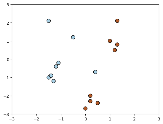
The above figure is a visualization of the 2D dataset we have created. We will then use it to illustrate the difference between various kernels.

14.3.2. Examples of Kernels#

14.3.2.1. Linear Kernel#

The simplest kind of kernel that exists is called the linear kernel. This simply corresponds to dot product multiplication of the features:

\[ K(x,z) = x^\top z \]

Applied to an SVM, this corresponds to a linear decision boundary.

Below is an example of how we can use the SVM implementation in sklearn with a linear kernel. Internally, this solves the dual SVM optimization problem.

# https://scikit-learn.org/stable/auto_examples/svm/plot_svm_kernels.html
clf = svm.SVC(kernel='linear' , gamma=2)
clf.fit(X, Y)

# plot the line, the points, and the nearest vectors to the plane
plt.scatter(clf.support_vectors_[:, 0], clf.support_vectors_[:, 1], s=80, facecolors='none', zorder=10, edgecolors='k')
plt.scatter(X[:, 0], X[:, 1], c=Y, zorder=10, cmap=plt.cm.Paired, edgecolors='k')
XX, YY = np.mgrid[x_min:x_max:200j, y_min:y_max:200j]
Z = clf.decision_function(np.c_[XX.ravel(), YY.ravel()])

# Put the result into a color plot
Z = Z.reshape(XX.shape)
plt.pcolormesh(XX, YY, Z > 0, cmap=plt.cm.Paired)
plt.contour(XX, YY, Z, colors=['k', 'k', 'k'], linestyles=['--', '-', '--'],levels=[-.5, 0, .5])
plt.xlim(x_min, x_max)
plt.ylim(y_min, y_max)

(-3.0, 3.0)

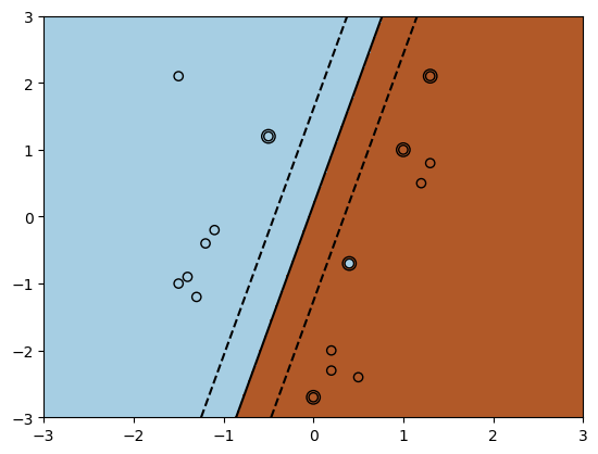
The above figure shows that a linear kernel provides linear decision boundaries to separate the data.

14.3.2.2. Polynomial Kernel#

A more interesting example is the polynomial kernel of degree $p$, of which we have already seen a simple example:

\[ K(x,z) = (x^\top z + c)^p. \]

This corresponds to a mapping to a feature space of dimension $d+p \choose p$ that has all monomials $x_{i_1}x_{i_2}\cdots x_{i_p}$ of degree at most $p$.

For $d=3$ this feature map looks like

\[\begin{split} \small \phi(x) = \begin{bmatrix} x_1 x_1 \\ x_1 x_2 \\ x_1 x_3 \\ x_2 x_1 \\ x_2 x_1 \\ x_2 x_2 \\ x_3 x_3 \\ x_3 x_1 \\ x_3 x_2 \\ x_3 x_3 \\ \sqrt{2}c x_1 \\ \sqrt{2}c x_2 \\ \sqrt{2}c x_3 \\ c \end{bmatrix}. \end{split}\]

The polynomial kernel allows us to compute dot products in a $O(d^p)$-dimensional space in time $O(d)$. The following code shows how it would be implemented in sklearn.

# https://scikit-learn.org/stable/auto_examples/svm/plot_svm_kernels.html
clf = svm.SVC(kernel='poly', degree=3, gamma=2)
clf.fit(X, Y)

# plot the line, the points, and the nearest vectors to the plane
plt.scatter(clf.support_vectors_[:, 0], clf.support_vectors_[:, 1], s=80, facecolors='none', zorder=10, edgecolors='k')
plt.scatter(X[:, 0], X[:, 1], c=Y, zorder=10, cmap=plt.cm.Paired, edgecolors='k')
XX, YY = np.mgrid[x_min:x_max:200j, y_min:y_max:200j]
Z = clf.decision_function(np.c_[XX.ravel(), YY.ravel()])

# Put the result into a color plot
Z = Z.reshape(XX.shape)
plt.pcolormesh(XX, YY, Z > 0, cmap=plt.cm.Paired)
plt.contour(XX, YY, Z, colors=['k', 'k', 'k'], linestyles=['--', '-', '--'],levels=[-.5, 0, .5])
plt.xlim(x_min, x_max)
plt.ylim(y_min, y_max)

(-3.0, 3.0)

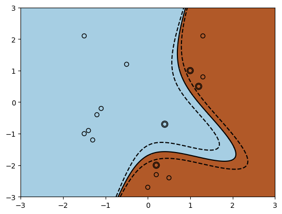
The above figure is a visualization of the polynomial kernel with degree of 3 and gamma of 2. The decision boundary is non-linear, in contrast to that of linear kernels.

14.3.2.3. Radial Basis Function Kernel#

Another example is the Radial Basis Function (RBF; sometimes called Gaussian) kernel

\[ K(x,z) = \exp \left(-\frac{||x - z||^2}{2\sigma^2}\right), \]

where $\sigma$ is a hyper-parameter. It’s easiest to understand this kernel by viewing it as a similarity measure.

We can show that this kernel corresponds to an infinite-dimensional feature map and the limit of the polynomial kernel as $p \to \infty$.

To see why that’s intuitively the case, consider the Taylor expansion

\[ \exp \left(-\frac{||x - z||^2}{2\sigma^2}\right) \approx 1 - \frac{||x - z||^2}{2\sigma^2} + \frac{||x - z||^4}{2! \cdot 4\sigma^4} - \frac{||x - z||^6}{3! \cdot 8\sigma^6} + \ldots \]

Each term on the right-hand side can be expanded into a polynomial. Thus, the above infinite series contains an infinite number of polynomial terms, and consequently an infinite number of polynomial features.

We can look at the sklearn implementation again.

# https://scikit-learn.org/stable/auto_examples/svm/plot_svm_kernels.html
clf = svm.SVC(kernel='rbf', gamma=.5)
clf.fit(X, Y)

# plot the line, the points, and the nearest vectors to the plane
plt.scatter(clf.support_vectors_[:, 0], clf.support_vectors_[:, 1], s=80, facecolors='none', zorder=10, edgecolors='k')
plt.scatter(X[:, 0], X[:, 1], c=Y, zorder=10, cmap=plt.cm.Paired, edgecolors='k')
XX, YY = np.mgrid[x_min:x_max:200j, y_min:y_max:200j]
Z = clf.decision_function(np.c_[XX.ravel(), YY.ravel()])

# Put the result into a color plot
Z = Z.reshape(XX.shape)
plt.pcolormesh(XX, YY, Z > 0, cmap=plt.cm.Paired)
plt.contour(XX, YY, Z, colors=['k', 'k', 'k'], linestyles=['--', '-', '--'],levels=[-.5, 0, .5])
plt.xlim(x_min, x_max)
plt.ylim(y_min, y_max)

(-3.0, 3.0)

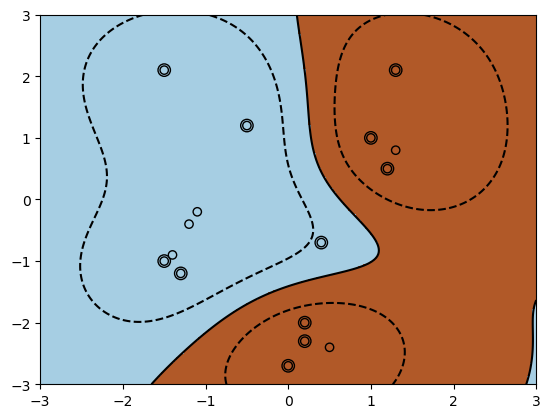
When using an RBF kernel, we may see multiple decision boundaries around different sets of points (as well as larger number of support vectors). These unusual shapes can be viewed as the projection of a linear max-margin separating hyperplane from a higher-dimensional (or infinite-dimensional) feature space into the original 2d space where $x$ lives.

There are even more kernel options in sklearn and we encourage you to try more of them using the same data.

14.3.3. When is $K$ A Kernel?#

We’ve seen that for many features $\phi$ we can define a kernel function $K : \mathcal{X} \times \mathcal{X} \to [0, \infty]$ that efficiently computes $\phi(x)^\top \phi(x)$. Suppose now that we use some kernel function $K : \mathcal{X} \times \mathcal{X} \to [0, \infty]$ in an ML algorithm. Is there an implicit feature mapping $\phi$ that corresponds to using K?

Let’s start by defining a necessary condition for $K : \mathcal{X} \times \mathcal{X} \to [0, \infty]$ to be associated with a feature map. Suppose that $K$ is a kernel for some feature map $\phi$, and consider an arbitrary set of $n$ points $\{x^{(1)}, x^{(2)}, \ldots, x^{(n)}\}$.

Consider the matrix $L \in \mathbb{R}^{n\times n}$ defined as $L_{ij} = K(x^{(i)}, x^{(j)}) = \phi(x^{(i)})^\top \phi(x^{(j)})$. We claim that $L$ must be symmetric and positive semidefinite. Indeed, $L$ is symmetric because the dot product $\phi(x^{(i)})^\top \phi(x^{(j)})$ is symmetric. Moreover, for any $z$,

\[\begin{split} \begin{align*} z^\top L z & = \sum_{i=1}^n \sum_{j=1}^n z_i L_{ij} z_j = \sum_{i=1}^n \sum_{j=1}^n z_i \phi(x^{(i)})^\top \phi(x^{(j)}) z_j \\ & = \sum_{i=1}^n \sum_{j=1}^n z_i (\sum_{k=1}^n \phi(x^{(i)})_k \phi(x^{(j)})_k ) z_j \\ & = \sum_{k=1}^n \sum_{i=1}^n \sum_{j=1}^n z_i \phi(x^{(i)})_k \phi(x^{(j)})_k z_j \\ & = \sum_{k=1}^n \sum_{i=1}^n \left( z_i \phi(x^{(i)})_k \right)^2 \geq 0 \end{align*} \end{split}\]

Thus if $K$ is a kernel, $L$ must be positive semidefinite for any $n$ points $x^{(i)}$.

14.3.3.1. Mercer’s Theorem#

The general idea of the theorem is that: if $K$ is a kernel, $L$ must be positive semidefinite for any set of $n$ points $x^{(i)}$. It turns out that it is is also a sufficient condition.

Theorem. (Mercer) Let $K: \mathcal{X} \times \mathcal{X} \to [0,\infty]$ be a kernel function. There exists a mapping $\phi$ associated with $K$ if for any $n$ and any dataset $\{x^{(1)}, x^{(2)}, \ldots, x^{(n)}\}$ of size $n \geq 1$, if and only if the matrix $L$ defined as $L_{ij} = K(x^{(i)}, x^{(j)})$ is symmetric and positive semidefinite.

This characterizes precisely which kernel functions correspond to some $\phi$.

14.3.4. Pros and Cons of Kernels#

We have introduce many good properties of kernels. However, are kernels a free lunch? Not quite.

Kernels allow us to use features $\phi$ of very large dimension $d$. However computation is at least $O(n^2)$, where $n$ is the dataset size. We need to compute distances $K(x^{(i)}, x^{(j)})$, for all $i,j$.

Approximate solutions can be found more quickly, but in practice kernel methods are not used with today’s massive datasets.
However, on small and medium-sized data, kernel methods will be at least as good as neural nets and probably much easier to train.

Examples of other algorithms in which we can use kernels include:

Supervised learning algorithms: linear regression, logistic regression, support vector machines, etc.
Unsupervised learning algorithms: PCA, density estimation.

Overall, kernels are very powerful because they can be used throughout machine learning.

Applied ML

Lecture 14: Kernels

Contents