Lecture 12: Support Vector Machines
Contents
Lecture 12: Support Vector Machines#
In this lecture, we are going to cover support vector machines (SVMs), one the most successful classification algorithms in machine learning.
12.1. Classification Margins#
We start the presentation of SVMs by defining the classification margin.
12.1.1. Review and Motivation#
12.1.1.1. Review of Binary Classification#
Consider a training dataset \(\mathcal{D} = \{(x^{(1)}, y^{(1)}), (x^{(2)}, y^{(2)}), \ldots, (x^{(n)}, y^{(n)})\}\). Recall that we distinguish between two types of supervised learning problems depending on the targets \(y^{(i)}\).
Regression: The target variable \(y \in \mathcal{Y}\) is continuous: \(\mathcal{Y} \subseteq \mathbb{R}\).
Binary Classification: The target variable \(y\) is discrete and takes on one of \(K=2\) possible values.
In this lecture, we focus on binary classification and assume \(\mathcal{Y} = \{-1, +1\}\).
Linear Model Family#
In this lecture, we will work with linear models of the form:
where \(x \in \mathbb{R}^d\) is a vector of features and \(y \in \{-1, 1\}\) is the target. The \(\theta_j\) are the parameters of the model. We can represent the model in a vectorized form as
12.1.1.2. Binary Classification Problem and The Iris Dataset#
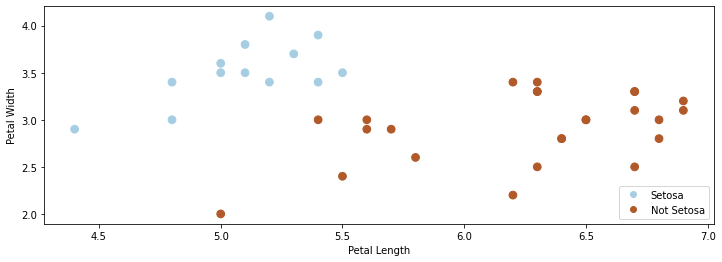
In this lecture, we will again use the Iris flower dataset. We will transform this problem into a binary classification task by merging the two non-Setosa flowers into one class. We use \(\mathcal{Y} =\{-1,1\}\) as the label space.
The resulting dataset is partly shown below.
import numpy as np
import pandas as pd
from sklearn import datasets

# Load the Iris dataset
iris = datasets.load_iris(as_frame=True)
iris_X, iris_y = iris.data, iris.target

# subsample to a third of the data points
iris_X = iris_X.loc[::4]
iris_y = iris_y.loc[::4]

# create a binary classification dataset with labels +/- 1
iris_y2 = iris_y.copy()
iris_y2[iris_y2==2] = 1
iris_y2[iris_y2==0] = -1

# print part of the dataset
pd.concat([iris_X, iris_y2], axis=1).head()
| sepal length (cm) | sepal width (cm) | petal length (cm) | petal width (cm) | target | |
|---|---|---|---|---|---|
| 0 | 5.1 | 3.5 | 1.4 | 0.2 | -1 |
| 4 | 5.0 | 3.6 | 1.4 | 0.2 | -1 |
| 8 | 4.4 | 2.9 | 1.4 | 0.2 | -1 |
| 12 | 4.8 | 3.0 | 1.4 | 0.1 | -1 |
| 16 | 5.4 | 3.9 | 1.3 | 0.4 | -1 |
As in earlier lectures, we visualize this dataset using matplotlib.
# https://scikit-learn.org/stable/auto_examples/neighbors/plot_classification.html
%matplotlib inline
import matplotlib.pyplot as plt
plt.rcParams['figure.figsize'] = [12, 4]
import warnings
warnings.filterwarnings("ignore")

# create 2d version of dataset and subsample it
X = iris_X.to_numpy()[:,:2]
x_min, x_max = X[:, 0].min() - .5, X[:, 0].max() + .5
y_min, y_max = X[:, 1].min() - .5, X[:, 1].max() + .5
xx, yy = np.meshgrid(np.arange(x_min, x_max, .02), np.arange(y_min, y_max, .02))

# Plot also the training points
p1 = plt.scatter(X[:, 0], X[:, 1], c=iris_y2, s=60, cmap=plt.cm.Paired)
plt.xlabel('Petal Length')
plt.ylabel('Petal Width')
plt.legend(handles=p1.legend_elements()[0], labels=['Setosa', 'Not Setosa'], loc='lower right')
<matplotlib.legend.Legend at 0x12b01cd30>
12.1.2. Comparing Classification Algorithms#
We have seen different types approaches to classification. When fitting a model, there may be many valid decision boundaries. How do we select one of them?
Consider the following three classification algorithms from sklearn. Each of them outputs a different classification boundary.
from sklearn.linear_model import LogisticRegression, Perceptron, RidgeClassifier
models = [LogisticRegression(), Perceptron(), RidgeClassifier()]

def fit_and_create_boundary(model):
    model.fit(X, iris_y2)
    Z = model.predict(np.c_[xx.ravel(), yy.ravel()])
    Z = Z.reshape(xx.shape)
    return Z

plt.figure(figsize=(12,3))
for i, model in enumerate(models):
    plt.subplot('13%d' % (i+1))
    Z = fit_and_create_boundary(model)
    plt.pcolormesh(xx, yy, Z, cmap=plt.cm.Paired)

    # Plot also the training points
    plt.scatter(X[:, 0], X[:, 1], c=iris_y2, edgecolors='k', cmap=plt.cm.Paired)
    plt.title('Algorithm %d' % (i+1))
    plt.xlabel('Sepal length')
    plt.ylabel('Sepal width')

plt.show()
12.1.2.1. Classification Scores#
Most classification algorithms output not just a class label but a score. For example, logistic regression returns the class probability
If the class probability is \(>0.5\), the model outputs class \(1\). The score is an estimate of confidence; it also represents how far we are from the decision boundary.
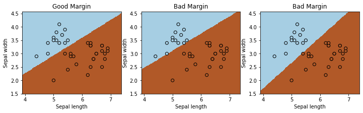
12.1.2.2. The Max-Margin Principle#
Intuitively, we want to select boundaries with high margin. This means that we are as confident as possible for every point and we are as far as possible from the decision boundary.
Several of the separating boundaries in our previous example had low margin: they came too close to the boundary.
from sklearn.linear_model import Perceptron, RidgeClassifier
from sklearn.svm import SVC
models = [SVC(kernel='linear', C=10000), Perceptron(), RidgeClassifier()]

def fit_and_create_boundary(model):
    model.fit(X, iris_y2)
    Z = model.predict(np.c_[xx.ravel(), yy.ravel()])
    Z = Z.reshape(xx.shape)
    return Z

plt.figure(figsize=(12,3))
for i, model in enumerate(models):
    plt.subplot('13%d' % (i+1))
    Z = fit_and_create_boundary(model)
    plt.pcolormesh(xx, yy, Z, cmap=plt.cm.Paired)

    # Plot also the training points
    plt.scatter(X[:, 0], X[:, 1], c=iris_y2, edgecolors='k', cmap=plt.cm.Paired)
    if i == 0:
        plt.title('Good Margin')
    else:
        plt.title('Bad Margin')
    plt.xlabel('Sepal length')
    plt.ylabel('Sepal width')

plt.show()
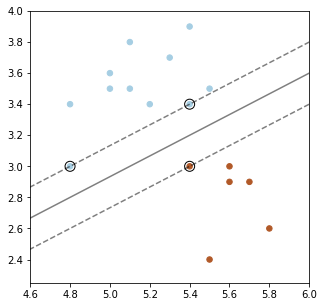
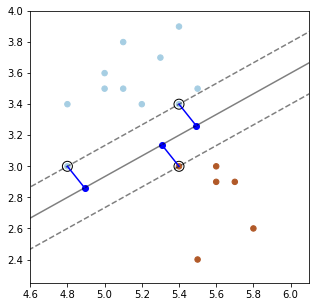
Below, we plot a decision boundary between the two classes (solid line) that has a high margin. The two dashed lines that lie at the margin.
Points that are the margin are highlighted in black. A good decision boundary is as far away as possible from the points at the margin.
#https://scikit-learn.org/stable/auto_examples/svm/plot_separating_hyperplane.html
from sklearn import svm

# fit the model, don't regularize for illustration purposes
clf = svm.SVC(kernel='linear', C=1000) # we'll explain this algorithm shortly
clf.fit(X, iris_y2)

plt.figure(figsize=(5,5))
plt.scatter(X[:, 0], X[:, 1], c=iris_y2, s=30, cmap=plt.cm.Paired)
Z = clf.decision_function(np.c_[xx.ravel(), yy.ravel()]).reshape(xx.shape)

# plot decision boundary and margins
plt.contour(xx, yy, Z, colors='k', levels=[-1, 0, 1], alpha=0.5,
           linestyles=['--', '-', '--'])
plt.scatter(clf.support_vectors_[:, 0], clf.support_vectors_[:, 1], s=100,
           linewidth=1, facecolors='none', edgecolors='k')
plt.xlim([4.6, 6])
plt.ylim([2.25, 4])
(2.25, 4.0)
12.1.3. The Functional Classification Margin#
How can we define the concept of margin more formally?
We can try to define the margin \(\tilde \gamma^{(i)}\) with respect to a training example \((x^{(i)}, y^{(i)})\) as
We call this the functional margin. Let’s analyze it.
We defined the functional margin as
If \(y^{(i)}=1\), then the margin \(\tilde\gamma^{(i)}\) is large when the model score \(f(x^{(i)}) = \theta^\top x^{(i)} + \theta_0\) is positive and large.
Thus, we are classifying \(x^{(i)}\) correctly and with high confidence.
If \(y^{(i)}=-1\), then the margin \(\tilde\gamma^{(i)}\) is large when the model score \(f(x^{(i)}) = \theta^\top x^{(i)} + \theta_0\) is negative and large in absolute value.
We are again classifying \(x^{(i)}\) correctly and with high confidence.
Thus higher margin means higher confidence at each input point. However, we have a problem.
If we rescale the parameters \(\theta, \theta_0\) by a scalar \(\alpha > 0\), we get new parameters \(\alpha \theta, \alpha \theta_0\) .
The \(\alpha \theta, \alpha \theta_0\) doesn’t change the classification of points.
However, the margin \(\left( \alpha \theta^\top x^{(i)} + \alpha \theta_0 \right) = \alpha \left( \theta^\top x^{(i)} + \theta_0 \right)\) is now scaled by \(\alpha\)!
It doesn’t make sense that the same classification boundary can have different margins when we rescale it.
12.1.4. The Geometric Classification Margin#
We define the geometric margin \(\gamma^{(i)}\) with respect to a training example \((x^{(i)}, y^{(i)})\) as
We call it geometric because \(\gamma^{(i)}\) equals the distance between \(x^{(i)}\) and the hyperplane.
We normalize the functional margin by \(||\theta||\)
Rescaling the weights does not make the margin arbitrarily large.
Let’s make sure our intuition about the margin holds.
If \(y^{(i)}=1\), then the margin \(\gamma^{(i)}\) is large when the model score \(f(x^{(i)}) = \theta^\top x^{(i)} + \theta_0\) is positive and large.
Thus, we are classifying \(x^{(i)}\) correctly and with high confidence.
The same holds when \(y^{(i)}=-1\). We again capture our intuition that increasing margin means increasing the confidence of each input point.
12.1.4.1. Geometric Intuitions#
The margin \(\gamma^{(i)}\) is called geometric because it corresponds to the distance from \(x^{(i)}\) to the separating hyperplane \(\theta^\top x + \theta_0 = 0\) (dashed line below).

Suppose that \(y^{(i)}=1\) (\(x^{(i)}\) lies on positive side of boundary). Then:
The points \(x\) that lie on the decision boundary are those for which \(\theta^\top x + \theta_0 = 0\) (score is precisely zero, and between 1 and -1).
The vector \(\frac{\theta}{||\theta||}\) is perpendicular to the hyperplane \(\theta^\top x + \theta_0\) and has unit norm (fact from calculus).
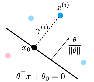
Let \(x_0\) be the point on the boundary closest to \(x^{(i)}\). Then by definition of the margin \(x^{(i)} = x_0 + \gamma^{(i)} \frac{\theta}{||\theta||}\) or
Since \(x_0\) is on the hyperplane, \(\theta^\top x_0 + \theta_0 = 0\), or
Solving for \(\gamma^{(i)}\) and using the fact that \(\theta^\top \theta = ||\theta||^2\), we obtain
Which is our geometric margin. The case of \(y^{(i)}=-1\) can also be proven in a similar way.
We can use our formula for \(\gamma\) to precisely plot the margins on our earlier plot.
# plot decision boundary and margins
plt.figure(figsize=(5,5))
plt.scatter(X[:, 0], X[:, 1], c=iris_y2, s=30, cmap=plt.cm.Paired)
plt.contour(xx, yy, Z, colors='k', levels=[-1, 0, 1], alpha=0.5,
           linestyles=['--', '-', '--'])
plt.scatter(clf.support_vectors_[:, 0], clf.support_vectors_[:, 1], s=100,
           linewidth=1, facecolors='none', edgecolors='k')
plt.xlim([4.6, 6.1])
plt.ylim([2.25, 4])

# plot margin vectors
theta = clf.coef_[0]
theta0 = clf.intercept_
for idx in clf.support_[:3]:
    x0 = X[idx]
    y0 = iris_y2.iloc[idx]
    margin_x0 = (theta.dot(x0) + theta0)[0] / np.linalg.norm(theta)
    w = theta / np.linalg.norm(theta)
    plt.plot([x0[0], x0[0]-w[0]*margin_x0], [x0[1], x0[1]-w[1]*margin_x0], color='blue')
    plt.scatter([x0[0]-w[0]*margin_x0], [x0[1]-w[1]*margin_x0], color='blue')
plt.show()
12.2. The Max-Margin Classifier#
We have seen a way to measure the confidence level of a classifier at a data point using the notion of a margin. Next, we are going to see how to maximize the margin of linear classifiers.
12.2.1. Maximizing the Margin#
We want to define an objective that will result in maximizing the margin. As a first attempt, consider the following optimization problem.
This maximises the smallest margin over the \((x^{(i)}, y^{(i)})\). It guarantees each point has margin at least \(\gamma\).
This problem is difficult to optimize because of the division by \(||\theta||\) and we would like to simplify it. First, consider the equivalent problem:
Note that this problem has an extra degree of freedom:
Suppose we multiply \(\theta, \theta_0\) by some constant \(c >0\).
This yields another valid solution!
To enforce uniqueness, we add another constraint that doesn’t change the minimizer:
This ensures we cannot rescale \(\theta\) and also asks our linear model to assign each \(x^{(i)}\) a score of at least \(\pm 1\):
If we constraint \(||\theta|| \cdot \gamma = 1\) holds, then we know that \(\gamma = 1/||\theta||\) and we can replace \(\gamma\) in the optimization problem to obtain:
The solution of this problem is still the same.
Finally, instead of maximizing \(1/||\theta||\), we can minimize \(||\theta||\), or equivalently we can minimize \(\frac{1}{2}||\theta||^2\).
This is now a quadratic program that can be solved using off-the-shelf optimization algorithms!
12.2.2. Algorithm: Linear Support Vector Machine Classification#
The above procedure describes the closed solution for Support Vector Machine. We can succinctly define the algorithm components.
Type: Supervised learning (binary classification).
Model family: Linear decision boundaries.
Objective function: Max-margin optimization.
Optimizer: Quadratic optimization algorithms.
Probabilistic interpretation: No simple interpretation!
Later, we will see several other versions of this algorithm.
12.3. Soft Margins and the Hinge Loss#
Let’s continue looking at how we can maximize the margin.
12.3.1. Non-Separable Problems#
So far, we have assume that a linear hyperplane exists. However, what if the classes are non-separable? Then our optimization problem does not have a solution and we need to modify it.
Our solution is going to be to make each constraint “soft”, by introducing “slack” variables, which allow the constraint to be violated.
If we can classify each point with a perfect score of \(\geq 1\), the \(\xi_i=0\).
If we cannot assign a perfect score, we assign a score of \(1-\xi_i\).
We define optimization such that the \(\xi_i\) are chosen to be as small as possible.
In the optimization problem, we assign a penalty \(C\) to these slack variables to obtain:
12.3.2. Towards an Unconstrained Objective#
Let’s further modify things. Moving around terms in the inequality we get:
If \(0 \geq 1 - y^{(i)}\left((x^{(i)})^\top\theta+\theta_0\right)\), we classified \(x^{(i)}\) perfectly and \(\xi_i = 0\)
If \(0 < 1 - y^{(i)}\left((x^{(i)})^\top\theta+\theta_0\right)\), then \(\xi_i = 1 - y^{(i)}\left((x^{(i)})^\top\theta+\theta_0\right)\)
Thus, \(\xi_i = \max\left(1 - y^{(i)}\left((x^{(i)})^\top\theta+\theta_0\right), 0 \right)\).
We simplify notation a bit by using the notation \((x)^+ = \max(x,0)\).
This yields:
Since \(\xi_i = \left(1 - y^{(i)}\left((x^{(i)})^\top\theta+\theta_0\right)\right)^+\), we can take
And we turn it into the following by plugging in the definition of \(\xi_i\):
Since it doesn’t matter which term we multiply by \(C>0\), this is equivalent to
for some \(\lambda > 0\).
We have now turned our optimizatin problem into an unconstrained form:
The hinge loss penalizes incorrect predictions.
The L2 regularizer ensures the weights are small and well-behaved.
12.3.3. The Hinge Loss#
Consider again our new loss term for a label \(y\) and a prediction \(f\):
Let’s examine the behavior of this loss on different \(y, f\):
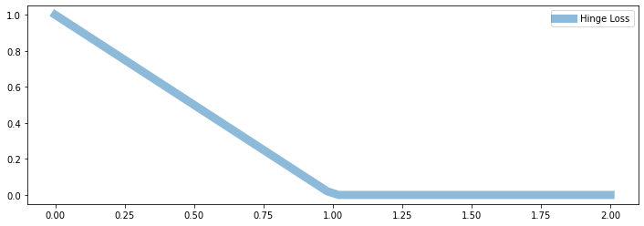
If prediction \(f\) has same sign as \(y\), and \(|f| \geq 1\), the loss is zero. In other words, if the class is correct, no penalty is applied if the absolute value of the score \(f\) is greater than 1.
However, if the prediction \(f\) is of the wrong sign, or \(|f| \leq 1\), the loss is \(|y - f|\). Thus, we penalize incorrect predictions, or predictions that are too close to the midpoint between the two class labels (which is at zero, since the labels are \(\pm 1\)).
Let’s visualize a few losses \(L(y=1,f)\), as a function of \(f\), including hinge.
# define the losses for a target of y=1
hinge_loss = lambda f: np.maximum(1 - f, 0)
l2_loss = lambda f: (1-f)**2
l1_loss = lambda f: np.abs(f-1)

# plot them
fs = np.linspace(0, 2)
plt.plot(fs, l1_loss(fs), fs, l2_loss(fs), fs, hinge_loss(fs), linewidth=9, alpha=0.5)
plt.legend(['L1 Loss', 'L2 Loss', 'Hinge Loss'])
plt.xlabel('Prediction f')
plt.ylabel('L(y=1,f)')
Text(0, 0.5, 'L(y=1,f)')
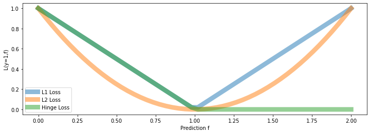
We can make a few interesting observations:
The hinge loss is linear like the L1 loss.
But it only penalizes errors that are on the “wrong” side:
We have an error of \(|f-y|\) if true class is \(1\) and \(f < 1\)
We don’t penalize for predicting \(f>1\) if true class is \(1\).
plt.plot(fs, hinge_loss(fs), linewidth=9, alpha=0.5)
plt.legend(['Hinge Loss'])
<matplotlib.legend.Legend at 0x12e750a58>
12.3.3.1. Properties of the Hinge Loss#
The hinge loss is one of the best losses in machine learning. We summarize here several important properties of the hinge loss.
It penalizes errors “that matter,” hence is less sensitive to outliers.
Minimizing a regularized hinge loss optimizes for a high margin.
The loss is non-differentiable at point, which may make it more challenging to optimize.
12.4. Optimization for SVMs#
We have seen a new way to formulate the SVM objective. Let’s now see how to optimize it.
12.4.0 Review#
12.4.0.1. Review: SVM Objective#
Maximizing the margin can be done in the following form:
The hinge loss penalizes incorrect predictions.
The L2 regularizer ensures the weights are small and well-behaved.
We can easily implement this objective in numpy.
First we define the model.
def f(X, theta):
    """The linear model we are trying to fit.

    Parameters:
    theta (np.array): d-dimensional vector of parameters
    X (np.array): (n,d)-dimensional data matrix

    Returns:
    y_pred (np.array): n-dimensional vector of predicted targets
    """
    return X.dot(theta)
And then we define the objective.
def svm_objective(theta, X, y, C=.1):
    """The cost function, J, describing the goodness of fit.

    Parameters:
    theta (np.array): d-dimensional vector of parameters
    X (np.array): (n,d)-dimensional design matrix
    y (np.array): n-dimensional vector of targets
    """
    return (np.maximum(1 - y * f(X, theta), 0) + C * 0.5 * np.linalg.norm(theta[:-1])**2).mean()
12.4.0.2. Review: Gradient Descent#
If we want to optimize \(J(\theta)\), we start with an initial guess \(\theta_0\) for the parameters and repeat the following update:
As code, this method may look as follows:
theta, theta_prev = random_initialization()
while norm(theta - theta_prev) > convergence_threshold:
    theta_prev = theta
    theta = theta_prev - step_size * gradient(theta_prev)
12.4.1. A Gradient for the Hinge Loss?#
What is the gradient for the hinge loss with a linear \(f\)?
Here, you see the linear part of \(J\) that behaves like \(1 - y \cdot f_\theta(x)\) (when \(y \cdot f_\theta(x) < 1\)) in orange:
plt.plot(fs, hinge_loss(fs),fs[:25], hinge_loss(fs[:25]), linewidth=9, alpha=0.5)
plt.legend(['Hinge Loss', 'Hinge Loss when $y \cdot f < 1$'])
<matplotlib.legend.Legend at 0x12ea6f940>
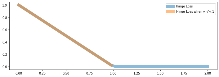
When \(y \cdot f_\theta(x) < 1\), we are in the “orange line” part and \(J(\theta)\) behaves like \(1 - y \cdot f_\theta(x)\).
Hence the gradient in this regime is:
where we used \(\nabla_\theta \theta^\top x = x\).
When \(y \cdot f_\theta(x) \geq 1\), we are in the “flat” part and \(J(\theta) = 0\). Hence the gradient is also just zero!
What is the gradient for the hinge loss with a linear \(f\)?
When \(y \cdot f_\theta(x) = 1\), we are in the “kink”, and the gradient is not defined!
In practice, we can either take the gradient when \(y \cdot f_\theta(x) > 1\) or the gradient when \(y \cdot f_\theta(x) < 1\) or anything in between. This is called the subgradient.
12.4.1.1. A Steepest Descent Direction for the Hinge Loss#
We can define a “gradient” like function \(\tilde \nabla_\theta J(\theta)\) for the hinge loss
It equals:
12.4.2. (Sub-)Gradient Descent for SVM#
Putting this together, we obtain a gradient descent algorithm (technically, it’s called subgradient descent).
theta, theta_prev = random_initialization()
while abs(J(theta) - J(theta_prev)) > conv_threshold:
    theta_prev = theta
    theta = theta_prev - step_size * approximate_gradient
Let’s implement this algorithm.
First we implement the approximate gradient.
def svm_gradient(theta, X, y, C=.1):
    """The (approximate) gradient of the cost function.

    Parameters:
    theta (np.array): d-dimensional vector of parameters
    X (np.array): (n,d)-dimensional design matrix
    y (np.array): n-dimensional vector of targets

    Returns:
    subgradient (np.array): d-dimensional subgradient
    """
    yy = y.copy()
    yy[y*f(X,theta)>=1] = 0
    subgradient = np.mean(-yy * X.T, axis=1)
    subgradient[:-1] += C * theta[:-1]
    return subgradient
And then we implement subgradient descent.
threshold = 5e-4
step_size = 1e-2

theta, theta_prev = np.ones((3,)), np.zeros((3,))
iter = 0
iris_X['one'] = 1
X_train = iris_X.iloc[:,[0,1,-1]].to_numpy()
y_train = iris_y2.to_numpy()

while np.linalg.norm(theta - theta_prev) > threshold:
    if iter % 1000 == 0:
        print('Iteration %d. J: %.6f' % (iter, svm_objective(theta, X_train, y_train)))
    theta_prev = theta
    gradient = svm_gradient(theta, X_train, y_train)
    theta = theta_prev - step_size * gradient
    iter += 1
Iteration 0. J: 3.728947
Iteration 1000. J: 0.376952
Iteration 2000. J: 0.359075
Iteration 3000. J: 0.351587
Iteration 4000. J: 0.344411
Iteration 5000. J: 0.337912
Iteration 6000. J: 0.331617
Iteration 7000. J: 0.326604
Iteration 8000. J: 0.322224
Iteration 9000. J: 0.319250
Iteration 10000. J: 0.316727
Iteration 11000. J: 0.314800
Iteration 12000. J: 0.313181
Iteration 13000. J: 0.311843
Iteration 14000. J: 0.310667
Iteration 15000. J: 0.309561
Iteration 16000. J: 0.308496
Iteration 17000. J: 0.307523
Iteration 18000. J: 0.306614
Iteration 19000. J: 0.305768
Iteration 20000. J: 0.305068
Iteration 21000. J: 0.304293
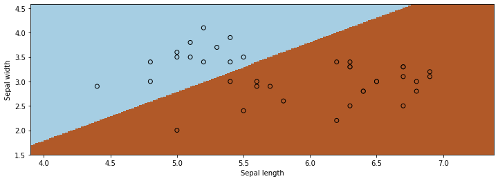
We can visualize the results to convince ourselves we found a good boundary.
xx, yy = np.meshgrid(np.arange(x_min, x_max, .02), np.arange(y_min, y_max, .02))
Z = f(np.c_[xx.ravel(), yy.ravel(), np.ones(xx.ravel().shape)], theta)
Z[Z<0] = 0
Z[Z>0] = 1

# Put the result into a color plot
Z = Z.reshape(xx.shape)
plt.pcolormesh(xx, yy, Z, cmap=plt.cm.Paired)

# Plot also the training points
plt.scatter(X_train[:, 0], X_train[:, 1], c=y_train, edgecolors='k', cmap=plt.cm.Paired)
plt.xlabel('Sepal length')
plt.ylabel('Sepal width')

plt.show()
12.4.3. Algorithm: Linear Support Vector Machine Classification#
The above procedure describes gradient descent optimization for support vector machines. The algorithm card below summarizes this algorithm and its components.
Type: Supervised learning (binary classification)
Model family: Linear decision boundaries.
Objective function: L2-regularized hinge loss.
Optimizer: Subgradient descent.
Probabilistic interpretation: No simple interpretation!