Congratulations on Finishing Applied Machine Learning!
You have made it! This is our last machine learning lecture, in which we will do an overview of the diffrent algorithms seen in the course.
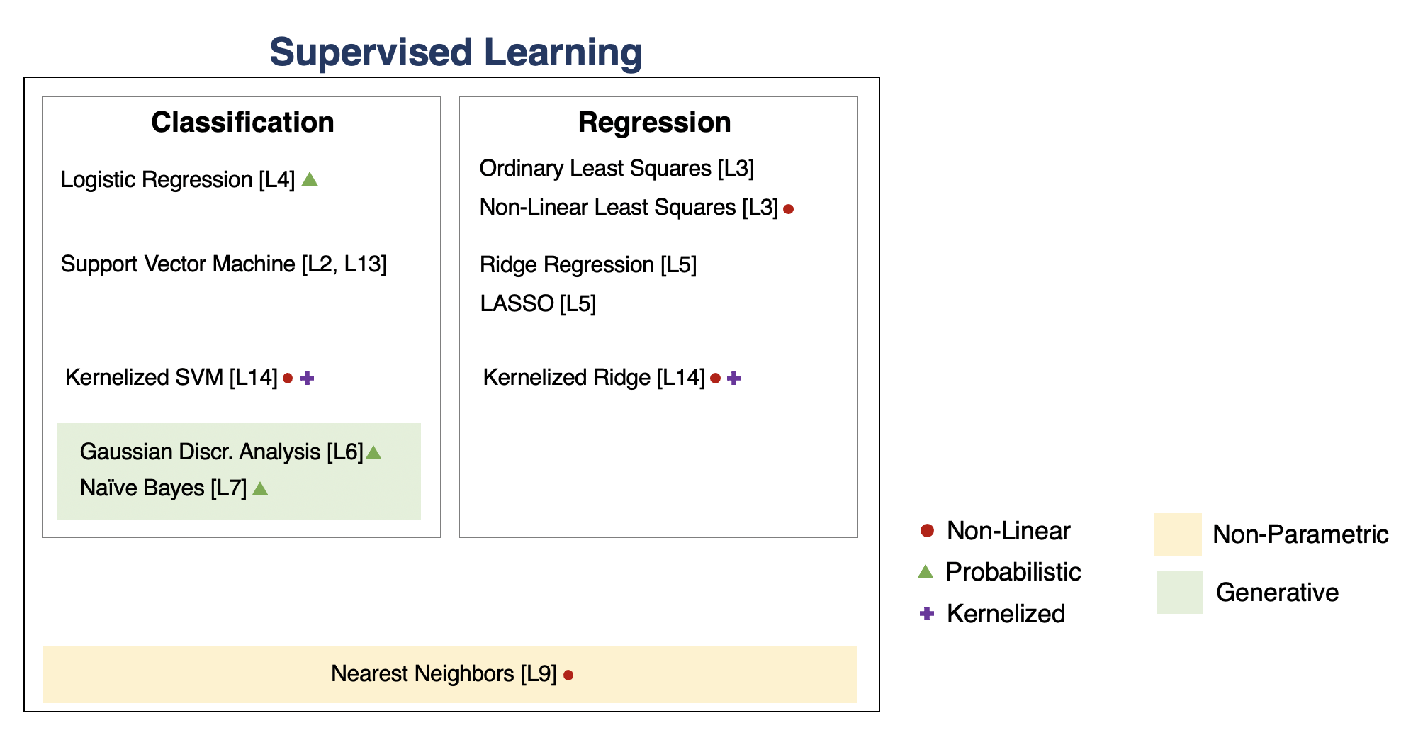
A Map of Applied Machine Learning
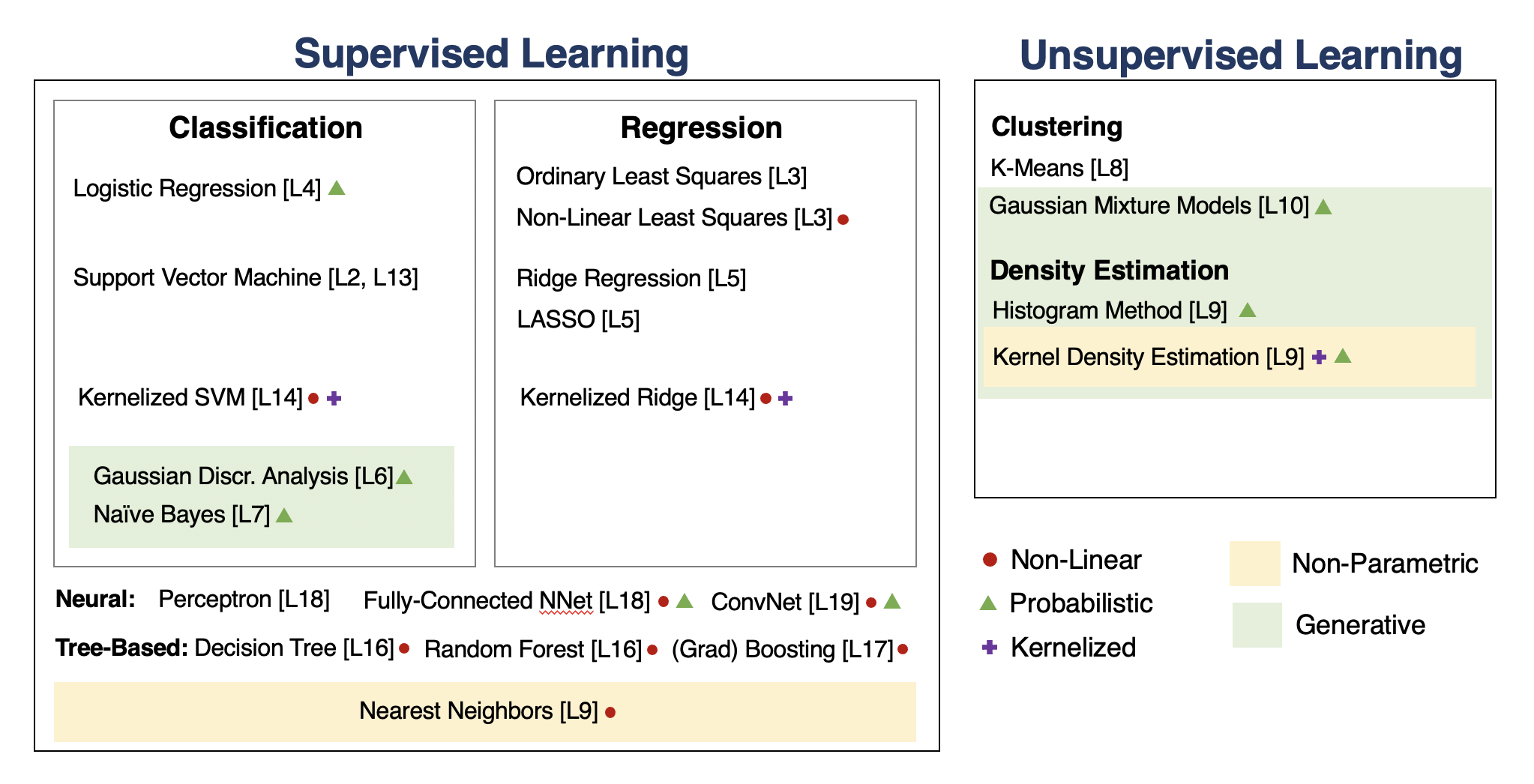
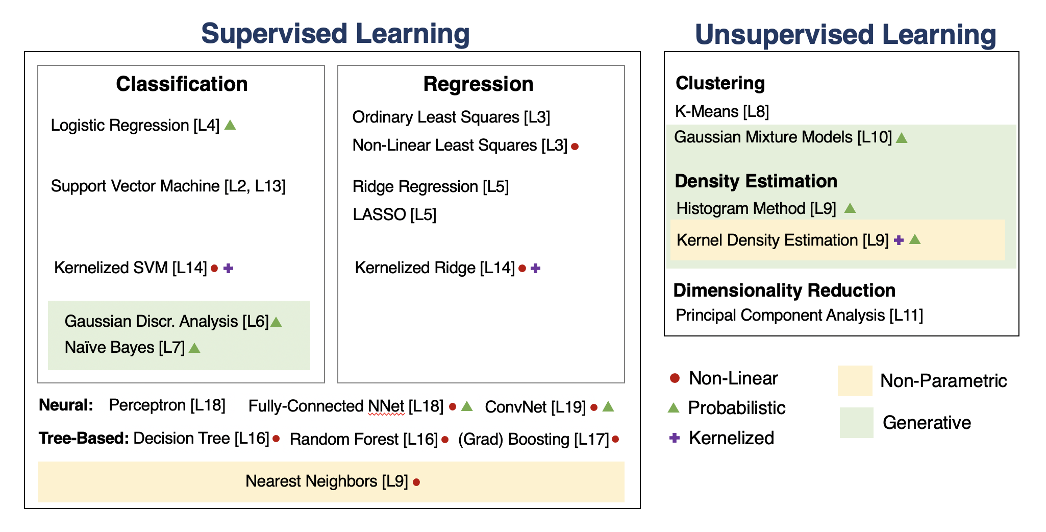
We will go through the following map of algorithms from the course.

Supervised Machine Learning
At a high level, a supervised machine learning problem has the following structure:
$$ \underbrace{\text{Dataset}}_\text{Features, Attributes} + \underbrace{\text{Learning Algorithm}}_\text{Model Class + Objective + Optimizer} \to \text{Predictive Model} $$The predictive model is chosen to model the relationship between inputs and targets. For instance, it can predict future targets.
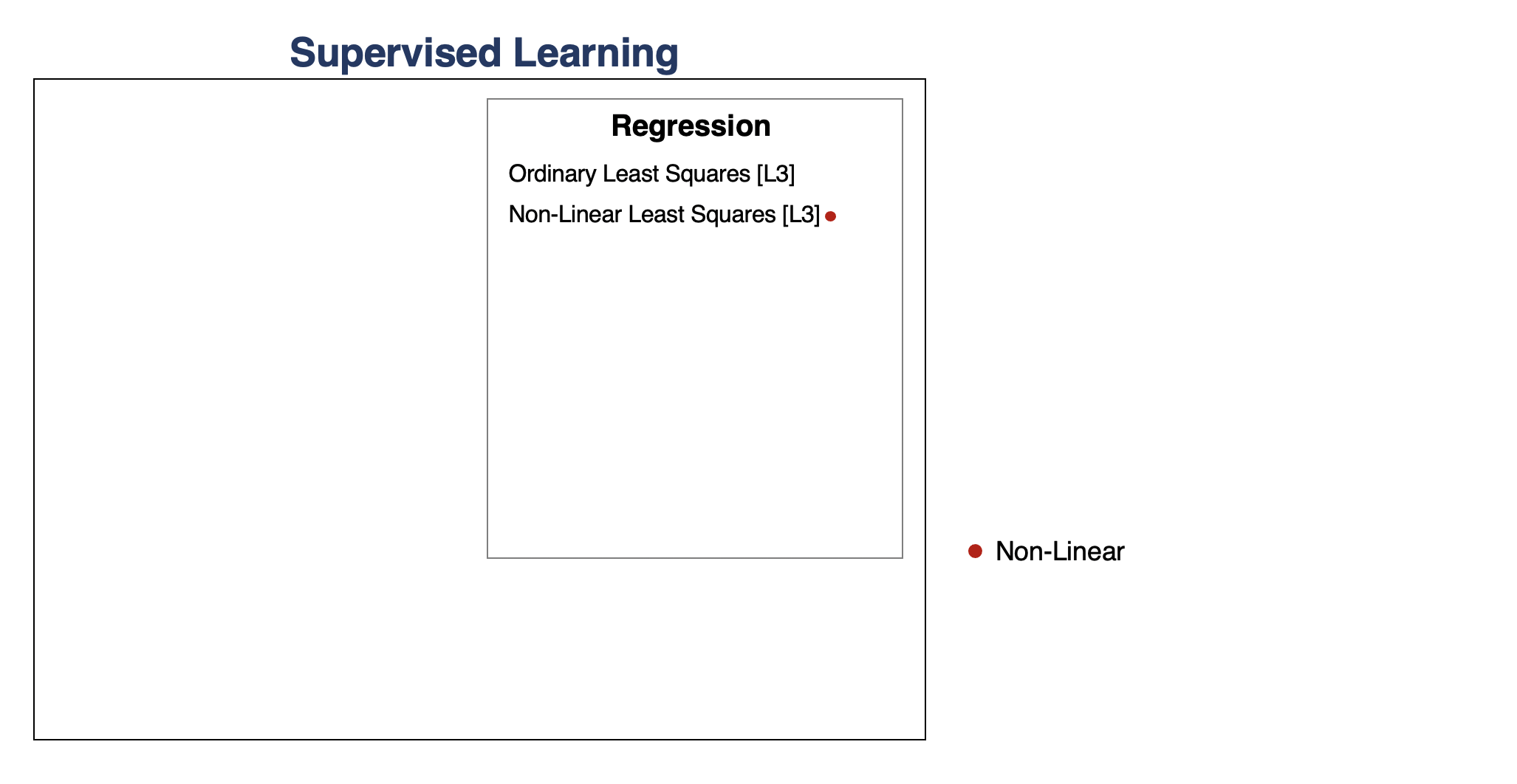
Linear Regression
In linear regression, we fit a model $$ f_\theta(x) := \theta^\top \phi(x) $$ that is linear in $\theta$.
The features $\phi(x) : \mathbb{R} \to \mathbb{R}^p$ are non-linear may non-linear in $x$ (e.g., polynomial features), allowing us to fit complex functions.
Overfitting
Overfitting is one of the most common failure modes of machine learning.
- A very expressive model (a high degree polynomial) fits the training dataset perfectly.
- The model also makes wildly incorrect prediction outside this dataset, and doesn't generalize.
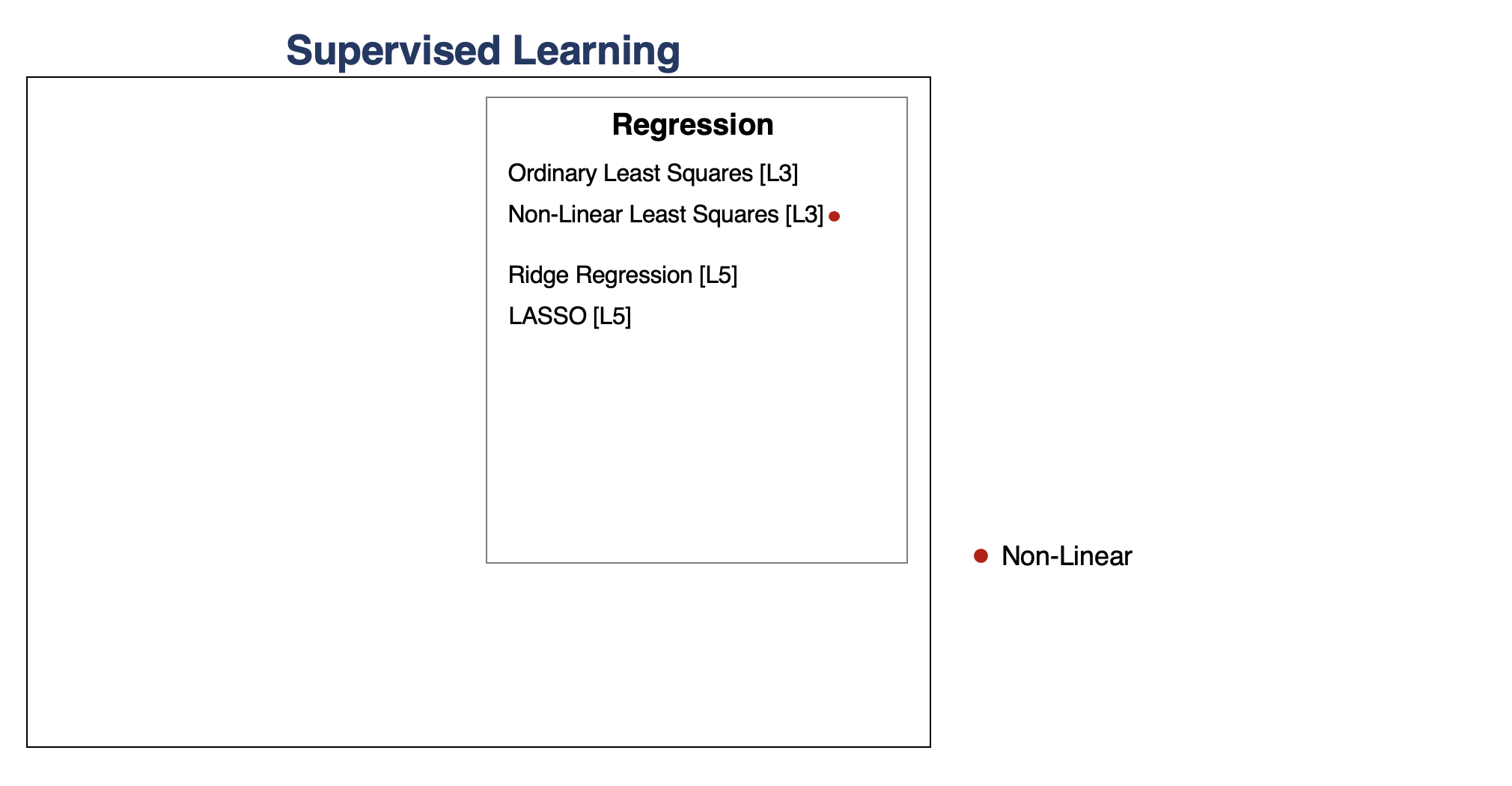
Regularization
The idea of regularization is to penalize complex models that may overfit the data.
Regularized least squares optimizes the following objective (Ridge). $$ J(\theta) = \frac{1}{2n} \sum_{i=1}^n \left( y^{(i)} - \theta^\top \phi(x^{(i)}) \right)^2 + \frac{\lambda}{2} \cdot ||\theta||_2^2. $$ If we use the L1 norm, we have the LASSO.
Regression vs. Classification
Consider a training dataset $\mathcal{D} = \{(x^{(1)}, y^{(1)}), (x^{(2)}, y^{(2)}), \ldots, (x^{(n)}, y^{(n)})\}$.
We distinguish between two types of supervised learning problems depnding on the targets $y^{(i)}$.
- Regression: The target variable $y \in \mathcal{Y}$ is continuous: $\mathcal{Y} \subseteq \mathbb{R}$.
- Classification: The target variable $y$ is discrete and takes on one of $K$ possible values: $\mathcal{Y} = \{y_1, y_2, \ldots y_K\}$. Each discrete value corresponds to a class that we want to predict.
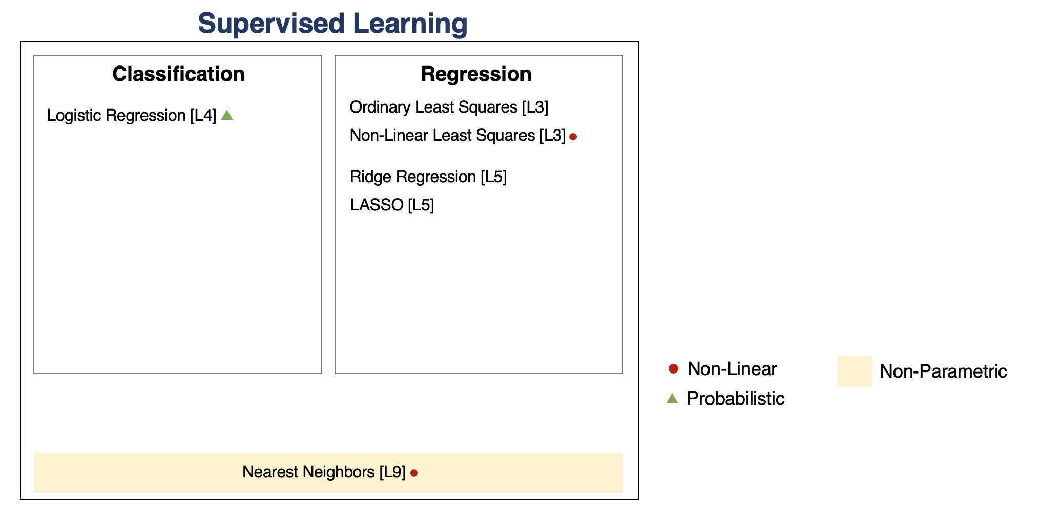
Parametric vs. Non-Parametric Models
Nearest neighbors is an example of a non-parametric model.
- A parametric model $f_\theta(x) : \mathcal{X} \times \Theta \to \mathcal{Y}$ is defined by a finite set of parameters $\theta \in \Theta$ whose dimensionality is constant with respect to the dataset
- In a non-parametric model, the function $f$ uses the entire training dataset to make predictions, and the complexity of the model increases with dataset size.
- Non-parametric models have the advantage of not loosing any information at training time.
- However, they are also computationally less tractable and may easily overfit the training set.
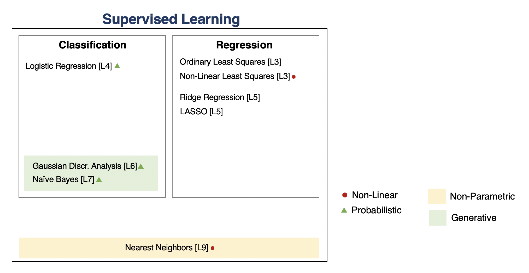
Probabilistic vs. Non-Probabilistic Models
A probabilistic model is a probability distribution $$P(x,y) : \mathcal{X} \times \mathcal{Y} \to [0,1].$$ This model can approximate the data distribution $P_\text{data}(x,y)$.
If we know $P(x,y)$, we can use the conditional $P(y|x)$ for prediction.
Maximum Likelihood Learning
Maximum likelihood is an objective that can be used to fit any probabilistic model: $$ \theta_\text{MLE} = \arg\max_\theta \mathbb{E}_{x, y \sim \mathbb{P}_\text{data}} \log P(x, y; \theta). $$ It minimizes the KL divergence between the model and data distributions: $$\theta_\text{MLE} = \arg\min_\theta \text{KL}(P_\text{data} \mid\mid P_\theta).$$
Discriminative vs. Generative Models
There are two types of probabilistic models: generative and discriminative. \begin{align*} \underbrace{P_\theta(x,y) : \mathcal{X} \times \mathcal{Y} \to [0,1]}_\text{generative model} & \;\; & \underbrace{P_\theta(y|x) : \mathcal{X} \times \mathcal{Y} \to [0,1]}_\text{discriminative model} \end{align*}
We can obtain predictions from generative models via $\max_y P_\theta(x,y)$.
The Max-Margin Principle
Intuitively, we want to select linear decision boundaries with high margin.
This means that we are as confident as possible for every point and we are as far as possible from the decision boundary.
import numpy as np
import pandas as pd
from sklearn import datasets

# Load the Iris dataset
iris = datasets.load_iris(as_frame=True)
iris_X, iris_y = iris.data, iris.target

# subsample to a third of the data points
iris_X = iris_X.loc[::4]
iris_y = iris_y.loc[::4]

# create a binary classification dataset with labels +/- 1
iris_y2 = iris_y.copy()
iris_y2[iris_y2==2] = 1
iris_y2[iris_y2==0] = -1

# print part of the dataset
pd.concat([iris_X, iris_y2], axis=1).head()
| sepal length (cm) | sepal width (cm) | petal length (cm) | petal width (cm) | target | |
|---|---|---|---|---|---|
| 0 | 5.1 | 3.5 | 1.4 | 0.2 | -1 |
| 4 | 5.0 | 3.6 | 1.4 | 0.2 | -1 |
| 8 | 4.4 | 2.9 | 1.4 | 0.2 | -1 |
| 12 | 4.8 | 3.0 | 1.4 | 0.1 | -1 |
| 16 | 5.4 | 3.9 | 1.3 | 0.4 | -1 |
# https://scikit-learn.org/stable/auto_examples/neighbors/plot_classification.html
%matplotlib inline
import matplotlib.pyplot as plt
plt.rcParams['figure.figsize'] = [12, 4]
import warnings
warnings.filterwarnings("ignore")

# create 2d version of dataset and subsample it
X = iris_X.to_numpy()[:,:2]
x_min, x_max = X[:, 0].min() - .5, X[:, 0].max() + .5
y_min, y_max = X[:, 1].min() - .5, X[:, 1].max() + .5
xx, yy = np.meshgrid(np.arange(x_min, x_max, .02), np.arange(y_min, y_max, .02))

# Plot also the training points
p1 = plt.scatter(X[:, 0], X[:, 1], c=iris_y2, s=60, cmap=plt.cm.Paired)
plt.xlabel('Petal Length')
plt.ylabel('Petal Width')
plt.legend(handles=p1.legend_elements()[0], labels=['Setosa', 'Not Setosa'], loc='lower right')
<matplotlib.legend.Legend at 0x12b41fb00>

from sklearn.linear_model import Perceptron, RidgeClassifier
from sklearn.svm import SVC
models = [SVC(kernel='linear', C=10000), Perceptron(), RidgeClassifier()]

def fit_and_create_boundary(model):
    model.fit(X, iris_y2)
    Z = model.predict(np.c_[xx.ravel(), yy.ravel()])
    Z = Z.reshape(xx.shape)
    return Z

plt.figure(figsize=(12,3))
for i, model in enumerate(models):
    plt.subplot('13%d' % (i+1))
    Z = fit_and_create_boundary(model)
    plt.pcolormesh(xx, yy, Z, cmap=plt.cm.Paired)

    # Plot also the training points
    plt.scatter(X[:, 0], X[:, 1], c=iris_y2, edgecolors='k', cmap=plt.cm.Paired)
    if i == 0:
        plt.title('Good Margin')
    else:
        plt.title('Bad Margin')
    plt.xlabel('Sepal length')
    plt.ylabel('Sepal width')

plt.show()


The Kernel Trick
Many algorithms in machine learning only involve dot products $\phi(x)^\top \phi(z)$ but not the features $\phi$ themselves.
We can often compute $\phi(x)^\top \phi(z)$ very efficiently for complex $\phi$ using a kernel function $K(x,z) = \phi(x)^\top \phi(z)$. This is the kernel trick.
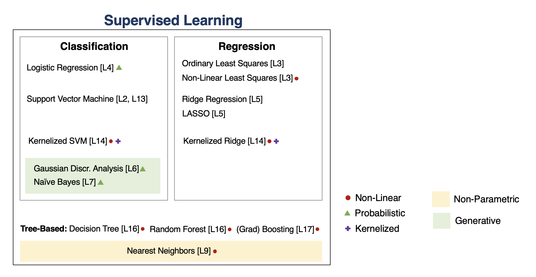
Tree-Based Models
Decision trees output target based on a tree of human-interpretable decision rules.
- Random forests combine large trees using bagging to reduce overfitting.
- Boosted trees combine small trees to reduce underfitting.
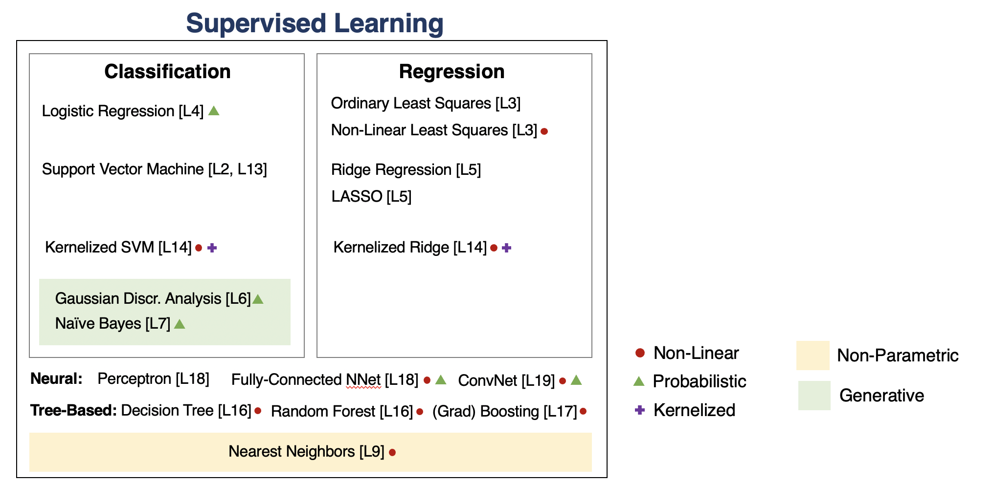
Neural Networks
Neural network models are inspired by the brain.
- A Perceptron is an artificial model of a neuron.
- MLP stack multiple layers of artifical neurons.
- ConvNets tie the weights of neighboring neurons into receptive fields that implement the convolution operation.
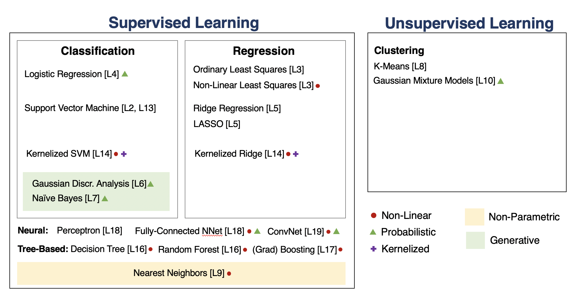
Unsupervised Learning
We have a dataset without labels. Our goal is to learn something interesting about the structure of the data:
- Clusters hidden in the dataset.
- A low-dimensional representation of the data.
- Recover the probability density that generated the data.
How To Decide Which Algorithm to Use
One factor is how much data you have. In the small data (<10,000) regime, consider:
- Linear models with hand-crafted features (LASSO, LR, NB, SVMs)
- Kernel methods often work best (e.g., SVM + RBF kernel)
- Non-parametric methods (kernels, nearest neighbors) are also powerful
In the big data regime,
- If using "high-level" features, gradient boosted trees are state-of-the-art
- When using "low-level" representations (images, sound signals), neural networks work best
- Linear models with good features are also good and reliable
Some additional advice:
- If interpretability matters, use decision trees or LASSO.
- When uncertainty estimates are important use probabilistic methods.
- If you know the data generating process, use generative models.
What's Next? Ideas for Courses
Consider the following courses to keep learning about ML:
- Graduate courses in the Spring semester at Cornell (generative models, NLP, etc.)
- Masters courses: Deep Learning Clinic, ML Engineering, Data Science, etc.
- Online courses, e.g. Full Stack Deep Learning
What's Next? Ideas for Research
In order to get involved in research, I recommend:
- Contacting research groups at Cornell for openings
- Watching online ML tutorials, e.g. NeurIPS
- Reading and implementing ML papers on your own
What's Next? Ideas for Industry Projects
Finally, a few ideas for how to get more practice applying ML in the real world:
- Participate in Kaggle competitions and review solutions
- Build an open-source project that you like and host it on Github
Thank You For Taking Applied Machine Learning!
