Part 1: Unsupervised Probabilistic Models
Density estimation is the problem of estimating a probability distribution from data.
As a first step, we will introduce probabilistic models for unsupervised learning.
Review: Unsupervised Learning
We have a dataset without labels. Our goal is to learn something interesting about the structure of the data:
- Clusters hidden in the dataset.
- Outliers: particularly unusual and/or interesting datapoints.
- Useful signal hidden in noise, e.g. human speech over a noisy phone.
Review: Data Distribution
We will assume that the dataset is sampled from a probability distribution $P_\text{data}$, which we will call the data distribution. We will denote this as $$x \sim P_\text{data}.$$
The dataset $\mathcal{D} = \{x^{(i)} \mid i = 1,2,...,n\}$ consists of independent and identicaly distributed (IID) samples from $P_\text{data}$.
Review: Unsupervised Models
We'll say that a model is a function $$ f : \mathcal{X} \to \mathcal{S} $$ that maps inputs $x \in \mathcal{X}$ to some notion of structure $s \in \mathcal{S}$.
Structure can have many definitions (clusters, low-dimensional representations, etc.), and we will see many examples.
Often, models have parameters $\theta \in \Theta$ living in a set $\Theta$. We will then write the model as $$ f_\theta : \mathcal{X} \to \mathcal{S} $$ to denote that it's parametrized by $\theta$.
Unsupervised Probabilistic Models
An unsupervised probabilistic model is a probability distribution $$P(x) : \mathcal{X} \to [0,1].$$ This model can approximate the data distribution $P_\text{data}$.
Probabilistic models also have parameters $\theta \in \Theta$, which we denote as $$P_\theta(x) : \mathcal{X} \to [0,1].$$
Why Use Probabilistic Models?
There are many tasks that we can solve with a good model $P_\theta$.
- Generation: sample new objects from $P_\theta$, such as images.
- Representation learning: find interesting structure in $P_\text{data}$
- Density estimation: approximate $P_\theta \approx P_\text{data}$ and use it to solve any downstream task (generation, clustering, outlier detection, etc.).
We are going to be interested in the latter.
Kullback-Leibler Divergence
In order to approximate $P_\text{data}$ with $P_\theta$, we need a measure of distance between distributions.
A standard measure of similarity between distributions is the Kullback-Leibler (KL) divergence between two distributions $p$ and $q$, defined as $$ D(p \| q) = \sum_{{\bf x}} p({\bf x}) \log \frac{p({\bf x})}{q({\bf x})}. $$
Observations:
- $D(p \, \| \, q) \geq 0$ for all $p, q$, with equality if and only if $p= q$. Proof:
\begin{align*}
D(p | q) = \mathbb{E}{x\sim p}{-\log \frac{q({\bf x})}{p({\bf x})}} & \geq -\log \left( \mathbb{E}{x\sim p} {\frac{q({\bf x})}{p({\bf x})}} \right) \ = &
-\log \left( \sum_{{\bf x}} p({\bf x}) \frac{q({\bf x})}{p({\bf x})} \right)
0 \end{align*} where in the first line we used Jensen's inequality
- The KL-divergence is asymmetric, i.e., $D(p \| q) \neq D(q \| p)$
From KL Divergence to Log Likelihood
$ \newcommand{\x}{x} \newcommand{\ex}[2]{\mathbb{E}_{#1 \sim #2}} \newcommand{\en}[2]{D(#1 \mid \mid #2)} $
We can learn $P_\theta$ that approximates $P_\text{data}$ by minimizing $D(P_{\textrm{data}} \mid \mid {P_\theta})$. This objective further simplifies as: \begin{eqnarray*} \en{P{\textrm{data}}}{P\theta} &=& \ex{\x}{P{\textrm{data}}}{\log\left( \frac{P{\textrm{data}}(\x)}{P\theta(\x)} \right)} \ &=& %-\bH(P{\textrm{data}}) \ex{\x}{P{\textrm{data}}}{\log P{\textrm{data}}(\x)}
- \ex{\x}{P{\textrm{data}}}{\log P\theta(\x)} \end{eqnarray*}
The first term does not depend on $P_\theta$: minimizing KL divergence is equivalent to maximizing the expected log-likelihood.
\begin{align*} \arg\min_{P_\theta} \en{P_{\textrm{data}}}{P_\theta} & = \arg\min_{P_\theta} - \ex{\x}{P_{\textrm{data}}}{\log P_\theta(\x)} \\ & = \arg\max_{P_\theta} \ex{\x}{P_{\textrm{data}}}{\log P_\theta(\x)} \end{align*}- This asks that $P_\theta$ assign high probability to instances sampled from $P_{\textrm{data}}$, so as to reflect the true distribution.
Problem: In general we do not know $P_{\textrm{data}}$, hence expected value is intractable.
Maximum Likelihood Estimation
$ \newcommand{\exd}[2]{\mathbb{E}_{#1 \sim #2}} \newcommand{\cd}{\mathcal{D}} $
Applying, Monte Carlo estimation, we may approximate the expected log-likelihood $$ \ex{\x}{P_{\textrm{data}}}{\log P_\theta(\x)} $$ with the empirical log-likelihood: $$ \exd{\cd}{P_\theta(\x)} = \frac{1}{|\cd|}\sum_{\x\in \cd} \log P_\theta(\x) $$
Maximum likelihood learning is then: $$ \max_{P_\theta} \hspace{2mm} \frac{1}{|\cd|}\sum_{\x\in \cd} \log P_\theta(\x). $$
Example: Flipping a Random Coin
How should we choose $P_\theta(x)$ if 3 out of 5 coin tosses are heads? Let's apply maximum likelihood learning.
- Our model is $P_\theta(x=H)=\theta$ and $P_\theta(x=T)=1-\theta$
- Our data is: $\cd=\{H,H,T,H,T\}$
- The likelihood of the data is $\prod_{i} P_\theta(x_i)=\theta \cdot \theta \cdot (1-\theta) \cdot \theta \cdot (1-\theta)$.
We optimize for $\theta$ which makes $\cd$ most likely. What is the solution in this case?
%matplotlib inline
import numpy as np
from matplotlib import pyplot as plt

# our dataset is {H, H, T, H, T}; if theta = P(x=H), we get:
coin_likelihood = lambda theta: theta*theta*(1-theta)*theta*(1-theta)

theta_vals = np.linspace(0,1)
plt.plot(theta_vals, coin_likelihood(theta_vals))
[<matplotlib.lines.Line2D at 0x1168f7390>]


Part 2: Kernel Density Estimation
Next, let's look at a first example of probabilistic models and how they are used to perform density estimation.
Review: Data Distribution
We will assume that the dataset is sampled from a probability distribution $\mathbb{P}$, which we will call the data distribution. We will denote this as $$x \sim P_\text{data}.$$
The dataset $\mathcal{D} = \{x^{(i)} \mid i = 1,2,...,n\}$ consists of independent and identicaly distributed (IID) samples from $P_\text{data}$.
Review: Unsupervised Probabilistic Models
An unsupervised probabilistic model is a probability distribution $$P_\theta(x) : \mathcal{X} \to [0,1].$$ This model can approximate the data distribution $P_\text{data}$. It may have parameters $\theta$.
Density Estimation
The problem of density estimation is to approximate the data distribution $P_\text{data}$ with the model $P$. $$ P \approx P_\text{data}. $$
It's also a general learning task. We can solve many downstream tasks using a good model $P$:
- Outlier and novelty detection
- Generating new samples $x$
- Visualizing and understanding the structure of $P_\text{data}$
Histogram Density Estimation
Perhaps the simplest approach to density estimation is by forming a histogram.
A histogram partitions the input space $x$ into a $d$-dimensional grid and counts the number of points in each cell.
This is best illustrated by an example.
Let's start by creating a simple 1D dataset coming from a mixture of two Gaussians:
$$P_\text{data}(x) = 0.3 \cdot \mathcal{N}(x ; \mu=0, \sigma=1) + 0.7 \cdot \mathcal{N}(x ; \mu=5, \sigma=1)$$# https://scikit-learn.org/stable/auto_examples/neighbors/plot_kde_1d.html
import numpy as np
np.random.seed(1)
N = 20 # number of points
# concat samples from two Gaussians:
X = np.concatenate((
np.random.normal(0, 1, int(0.3 * N)),
np.random.normal(5, 1, int(0.7 * N))
))[:, np.newaxis]
bins = np.linspace(-5, 10, 10) # locations of the bins
# print out X
print(X.flatten())
[ 1.62434536 -0.61175641 -0.52817175 -1.07296862  0.86540763 -2.3015387
  6.74481176  4.2387931   5.3190391   4.75062962  6.46210794  2.93985929
  4.6775828   4.61594565  6.13376944  3.90010873  4.82757179  4.12214158
  5.04221375  5.58281521]
We can now estimate the density using a histogram.
import matplotlib.pyplot as plt

plt.hist(X[:, 0], bins=bins, density=True) # plot the histogram
plt.plot(X[:, 0], np.full(X.shape[0], -0.01), '.k', markersize=10) # plot the points in X
plt.xlim(-4, 9)
plt.ylim(-0.02, 0.25)
(-0.02, 0.25)

Limitations of Histograms
Histogram-based methods have a number of shortcomings.
- The number of grid cells increases exponentially with dimension $d$.
- The histogram is not "smooth".
- The shape of the histogram depends on the bin positions.
We will now try to address the last two limitations.
Let's also visualize what we mean when we say that shape of the histogram depends on the histogram bins.
fig, ax = plt.subplots(1, 2, sharex=True, sharey=True, figsize=(12,4))
ax[0].hist(X[:, 0], bins=bins, density=True) # plot the histogram
ax[1].hist(X[:, 0], bins=bins+0.75, density=True) # plot the histogram with bin centers shifted by 0.75
for axi in ax.ravel():
    axi.plot(X[:, 0], np.full(X.shape[0], -0.01), '.k', markersize=10) # plot the points in X
    axi.set_xlim(-4, 9)
    axi.set_ylim(-0.02, 0.3)

Kernel Density Estimation: Idea
Kernel density estimation (KDE) is a different approach to histogram estimation.
- A histogram has $b$ bins of width $\delta$ at fixed positions.
- KDE effectively places a bin of with $\delta$ at each $x \in \mathcal{X}$.
- To obtain $P(x)$, we count the % of points that fall in the bin centered at $x$.
Tophat Kernel Density Estimation
The simplest form of this strategy (Tophat KDE) assumes a model of the form $$P_\delta(x) = \frac{N(x; \delta)}{n},$$ where $$ N(x; \delta) = |\{x^{(i)} : ||x^{(i)} - x || \leq \delta/2\}|, $$ is the number of points that are within a bin of with $\delta$ centered at $x$.
This is best understood via a picture.
from sklearn.neighbors import KernelDensity

kde = KernelDensity(kernel='tophat', bandwidth=0.75).fit(X) # fit a KDE model
x_ticks = np.linspace(-5, 10, 1000)[:, np.newaxis] # choose 1000 points on x-axis
log_density = kde.score_samples(x_ticks) # compute density at 1000 points

plt.fill(x_ticks[:, 0], np.exp(log_density)) # plot the density estimate
plt.plot(X[:, 0], np.full(X.shape[0], -0.01), '.k', markersize=10) # plot the points in X
plt.xlim(-4, 9)
plt.ylim(-0.02, 0.32)
(-0.02, 0.32)

The above algorithm still has the problem of producing a density estimate that is not smooth.
We are going to resolve this by replacing histogram counts with weighted averages.
Review: Kernels
A kernel function $K : \mathcal{X} \times \mathcal{X} \to [0, \infty]$ maps pairs of vectors $x, z \in \mathcal{X}$ to a real-valued score $K(x,z)$.
- A kernel represents the similarity between $x$ and $z$.
- It also often encodes the dot product between $x$ and $z$ in some high-dimensional feature space
We will use the first interpretation here.
Kernel Density Estimation
A kernelized density model $P$ takes the form: $$P(x) \propto \sum_{i=1}^n K(x, x^{(i)}).$$ This can be interpreted in different ways:
- We count the number of points "near" $x$, but each $x^{(i)}$ has a weight $K(x, x^{(i)})$ that depends on similarity between $x, x^{(i)}$.
- We place a "micro-density" $K(x, x^{(i)})$ at each $x^{(i)}$; the final density $P(x)$ is their sum.
Types of Kernels
We have seen several types of kernels in the context of support vector machines.
There are additional kernels that are popular for density estimation.
The following kernels are available in scikit-learn.
- Gaussian kernel $K(x,z; \delta) \propto \exp(-||x-z||^2/2\delta^2)$
- Tophat kernel $K(x,z; \delta) = 1 \text{ if } ||x-z|| \leq \delta/2$ else $0$.
- Epanechnikov kernel $K(x,z; \delta) \propto 1 - ||x-z||^2/\delta^2$
- Exponential kernel $K(x,z; \delta) \propto \exp(-||x-z||/\delta)$
- Linear kernel $K(x,z; \delta) \propto (1 - ||x-z||/\delta)^+$
It's easier to understand these kernels by looking at a figure.
# https://scikit-learn.org/stable/auto_examples/neighbors/plot_kde_1d.html
X_plot = np.linspace(-6, 6, 1000)[:, None]
X_src = np.zeros((1, 1))

fig, ax = plt.subplots(2, 3, sharex=True, sharey=True, figsize=(12,4))
fig.subplots_adjust(left=0.05, right=0.95, hspace=0.05, wspace=0.05)

def format_func(x, loc):
    if x == 0:
        return '0'
    elif x == 1:
        return '$\delta/2$'
    elif x == -1:
        return '-$\delta/2$'
    else:
        return '%i$\delta$' % (int(x/2))

for i, kernel in enumerate(['gaussian', 'tophat', 'epanechnikov',
                            'exponential', 'linear', 'cosine']):
    axi = ax.ravel()[i]
    log_dens = KernelDensity(kernel=kernel).fit(X_src).score_samples(X_plot)
    axi.fill(X_plot[:, 0], np.exp(log_dens), '-k', fc='#AAAAFF')
    axi.text(-2.6, 0.95, kernel)

    axi.xaxis.set_major_formatter(plt.FuncFormatter(format_func))
    axi.xaxis.set_major_locator(plt.MultipleLocator(1))
    axi.yaxis.set_major_locator(plt.NullLocator())

    axi.set_ylim(0, 1.05)
    axi.set_xlim(-2.9, 2.9)

ax[0, 1].set_title('Available Kernels')
Text(0.5, 1.0, 'Available Kernels')

Kernel Density Estimation: Example
Let's look at an example in the context of the 1D points we have seen earlier.
We will fit a model of the form $$P(x) = \sum_{i=1}^n K(x, x^{(i)})$$ with a Gaussian kernel $K(x,z; \delta) \propto \exp(-||x-z||^2/2\delta^2)$.
from sklearn.neighbors import KernelDensity

kde = KernelDensity(kernel='gaussian', bandwidth=0.75).fit(X) # fit a KDE model
x_ticks = np.linspace(-5, 10, 1000)[:, np.newaxis] # choose 1000 points on x-axis
log_density = kde.score_samples(x_ticks) # compute density at 1000 points
gaussian_kernel = lambda z : lambda x: np.exp(-np.abs(x-z)**2/(0.75**2)) # gaussian kernel
kernel_linspace = lambda x : np.linspace(x-1.2,x+1.2,30)

plt.figure(figsize=(12,4))
plt.plot(x_tick s[:, 0], np.exp(log_density)) # plot the density estimate
plt.plot(X[:, 0], np.full(X.shape[0], -0.01), '.k', markersize=10) # plot the points in X
plt.plot(kernel_linspace(4), 0.07*gaussian_kernel(4)(kernel_linspace(4)), '--', color='r', alpha=0.75)
plt.plot(kernel_linspace(5), 0.07*gaussian_kernel(5)(kernel_linspace(5)), '--', color='r', alpha=0.75)
plt.plot(kernel_linspace(1), 0.07*gaussian_kernel(1)(kernel_linspace(1)), '--', color='r', alpha=0.75)
plt.xlim(-4, 9)
plt.ylim(-0.02, 0.32)
(-0.02, 0.32)

KDE in Higher Dimensions
In priciple, kernel density estimation also works in higher dimensions.
However, the number of datapoints needed for a good fit incrases expoentially with the dimension, which limits the applications of this model in high dimensions.
Choosing Hyperparameters
Each kernel has a notion of "bandwidth" $\delta$. This is a hyperparameter that controls the "smoothness" of the fit.
- We can choose it using inspection or heuristics like we did for $K$ in $K$-Means.
- Because we have a probabilistic model, we can also estimate likelihood on a holdout dataset (more on this later!)
Let's illustrate how the bandwidth affects smoothness via an example.
from sklearn.neighbors import KernelDensity

kde1 = KernelDensity(kernel='gaussian', bandwidth=3).fit(X) # fit a KDE model
kde2 = KernelDensity(kernel='gaussian', bandwidth=0.2).fit(X) # fit a KDE model

fig, ax = plt.subplots(1, 2, sharex=True, sharey=True, figsize=(12,4))
ax[0].fill(x_ticks[:, 0], np.exp(kde1.score_samples(x_ticks))) # plot the density estimate
ax[1].fill(x_ticks[:, 0], np.exp(kde2.score_samples(x_ticks))) # plot the density estimate
ax[0].set_title('Bandwidth Too High')
ax[1].set_title('Bandwidth Too Low')

for axi in ax.ravel():
    axi.plot(X[:, 0], np.full(X.shape[0], -0.01), '.k', markersize=10) # plot the points in X
    axi.set_xlim(-4, 9)
    axi.set_ylim(-0.02, 0.4)

Algorithm: Kernel Density Estimation
- Type: Unsupervised learning (density estimation).
- Model family: Non-parametric. Sum of $n$ kernels.
- Objective function: Log-likelihood to choose optimal bandwidth.
- Optimizer: Grid search.
Pros and Cons of KDE
Pros:
- Can approximate any data distribution arbtrarily well.
Cons:
- Need to store entire dataset to make queries, which is computationally prohibitive.
- Number of data needed scale exponentially with dimension ("curse of dimensionality").
Part 3: Latent Variable Models
Probabilistic models we have seen earlier often need to approximate complex distributions.
In order to make our models more expressive, we introduce additional structure in the form of latent variables.
Review: Probabilistic Models
An unsupervised probabilistic model is a probability distribution $$P(x) : \mathcal{X} \to [0,1].$$ This model can approximate the data distribution $P_\text{data}$.
Probabilistic models also have parameters $\theta \in \Theta$, which we denote as $$P_\theta(x) : \mathcal{X} \to [0,1].$$
Review: Maximum Likelihood
In maximum likelihood learning, we maximize the empirical log-likelihood $$ \max_{P_\theta} \hspace{2mm} \frac{1}{|\cd|}\sum_{\x\in \cd} \log P_\theta(\x), $$ where $\mathcal{D} = \{x^{(i)} \mid i = 1,2,...,n\}$ is a dataset of independent and identicaly distributed (IID) samples from $P_\text{data}$.
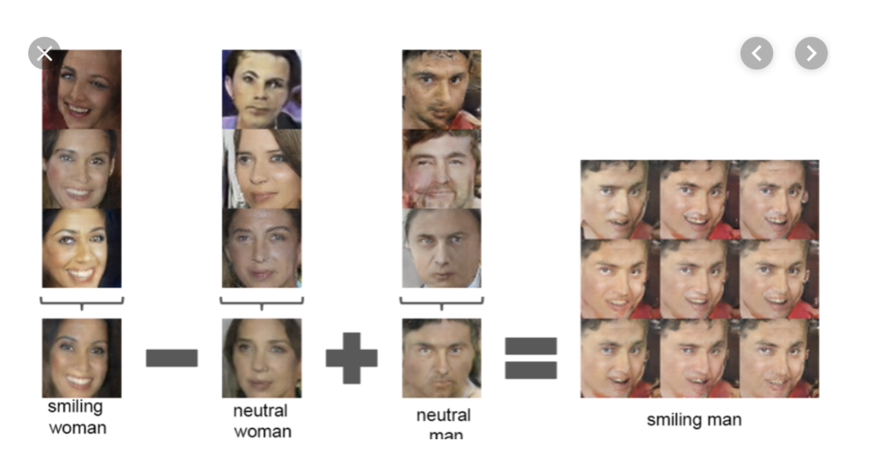
Latent Variable Models: Motivation
Consider the following dataset of human faces.
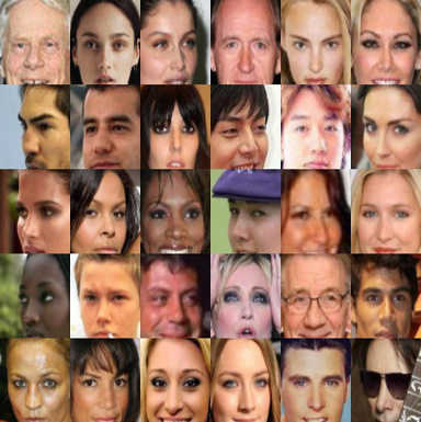
- It contains variability due to gender, eye color, hair color, pose, etc.
- However, unless these images are annotated, these factors of variation are not explicitly available (latent).
Idea: Explicitly model these factors using latent variables $z$
Latent Variable Models: Definition
An latent-variable model is a probability distribution $$P_\theta(x, z) : \mathcal{X} \times \mathcal{Z} \to [0,1]$$
containing two sets of variables:
- Observed $x$ that represent the high-dimensional object we are trying to model.
- Latent $z$ that are not in the training set, but can encode hidden structure in the data.
This model defines a $P_\theta(x) = \sum_{z \in \mathcal{Z}} P_\theta(x,z)$ that can approximate the data distribution $P_\text{data}(x)$.
Latent Variable Models: Example
Consider the following example of latent variables
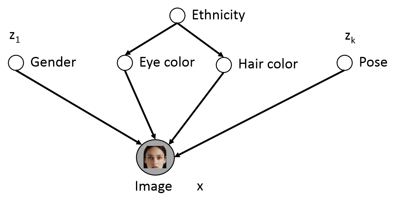
Only shaded variables $x$ are observed in the data (pixel values). Latent variables $z$ correspond to high level features
- If $z$ is chosen properly, $\Pr(x| z)$ is much simpler than $\Pr(x)$
- We can identify features via $\Pr(z \mid x)$, e.g., $\Pr(\text{eye color} = \text{blue} | \x)$
Mixtures of Gaussians
A mixture of Gaussians is a probability distribution $P(x,z)$ that factorizes into two components:
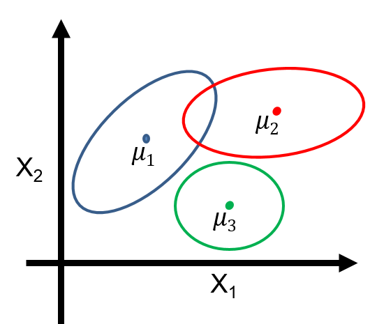
- $P_\theta(z)$ is a categorical distribution, and $P_\theta(z=k) = \phi_k$.
- $P_\theta(x\mid z=k)$ is a multivariate Gaussian $\mathcal{N}(x; \mu_k, \Sigma_k)$ with mean and covariance $\mu_k, \Sigma_k$.
Thus, $P_\theta(x,z)$ is a mixture of $K$ Gaussians: $$P_\theta(x,z) = \sum_{k=1}^K P_\theta(z=k) P_\theta(x|z=k) = \sum_{k=1}^K \phi_k \mathcal{N}(x; \mu_k, \Sigma_k)$$
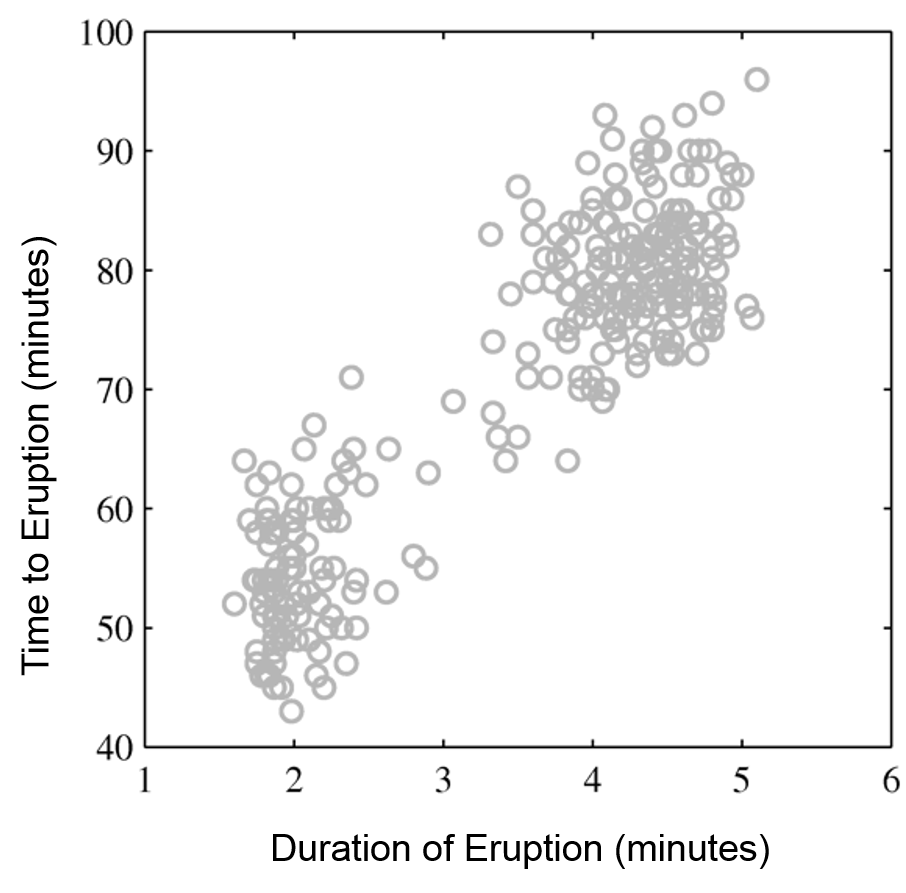
Mixtures of Gaussians fit more complex distributions than one Gaussian.
| Raw data | Single Gaussian | Mixture of Gaussians |
|---|---|---|
 |
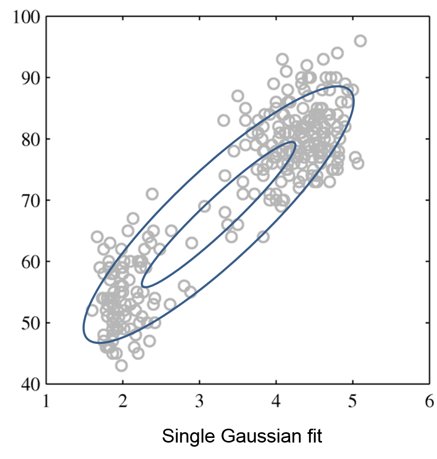 |
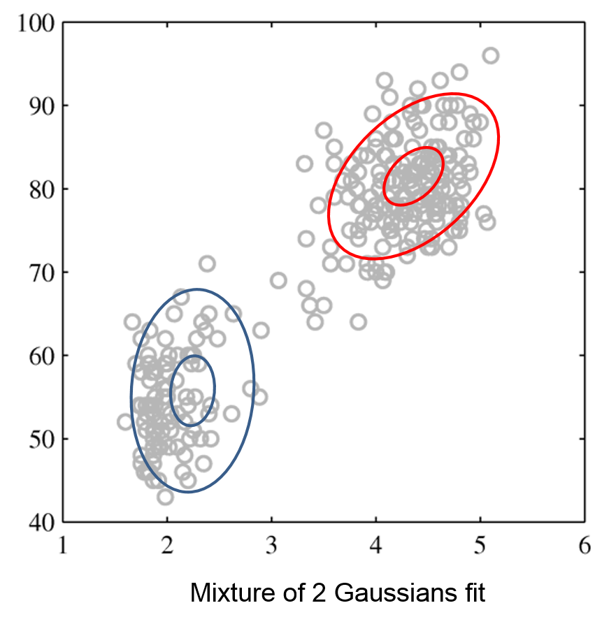 |
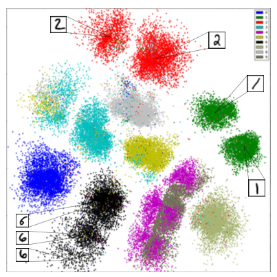
Feature Representations from LVMs
Given $P_\theta(x,z)$ we can compute $P_\theta(z|x)$ to find useful latent representations.
Latent variables are also useful to identify clusters in the data.
Learning Latent Variable Models
We can learn latent variable models using maximum likelihood: $$ \sum_{\x\in \cd} \log \Pr(\x ; \theta) = \sum_{\x\in \cd} \log \sum_{z \in \mathcal{Z}}\Pr(\x, z; \theta) $$
However, optimizing this objective is almost always intractable.
- Consider a latent variable $z \in \{0,1\}^{30}$, of thirty binary dimensions.
- We need to sum over $2^{30} \approx$ 1B possible values that $z$ can take.
- For continuous variables we may need to solve an intractable integral $\int P(x,z) dz$.
Approximate Inference in LVMs
In practice, we need to compute the likelihood objective (and its gradients) approximately.
- This is called approximate inference. We will see examples soon.
- The alternating algorithm for K-Means was a first simple example.
Summary of LVMs
Latent-variable models are an important class of machine learning models.
- They can represent complex probability distributions
- They can find unsupervised feature representations
They also have drawbacks:
- Learning these models is computationally intractable and requires approximate algorithms
- Computing $P(z|x)$ to obtain latent features is also often intractable.