Part 1: What is Unsupervised Learning?
Let's start by understanding what is unsupervised learning at a high level, starting with a dataset and an algorithm.
Unsupervised Learning
We have a dataset without labels. Our goal is to learn something interesting about the structure of the data:
- Clusters hidden in the dataset.
- Outliers: particularly unusual and/or interesting datapoints.
- Useful signal hidden in noise, e.g. human speech over a noisy phone.
Components of Unsupervised Learning
At a high level, an unsupervised machine learning problem has the following structure:
$$ \text{Dataset} + \text{Algorithm} \to \text{Unsupervised Model} $$The unsupervised model describes interesting structure in the data. For instance, it can identify interesting hidden clusters.
An Unsupervised Learning Dataset
As a first example of an unsupervised learning dataset, we will use our Iris flower example, but we will discard the labels.
We start by loading this dataset.
# import standard machine learning libraries
import numpy as np
import pandas as pd
from sklearn import datasets

# Load the Iris dataset
iris = datasets.load_iris()

print(iris.DESCR)
.. _iris_dataset:

Iris plants dataset
--------------------

**Data Set Characteristics:**

    :Number of Instances: 150 (50 in each of three classes)
    :Number of Attributes: 4 numeric, predictive attributes and the class
    :Attribute Information:
        - sepal length in cm
        - sepal width in cm
        - petal length in cm
        - petal width in cm
        - class:
                - Iris-Setosa
                - Iris-Versicolour
                - Iris-Virginica

    :Summary Statistics:

    ============== ==== ==== ======= ===== ====================
                    Min  Max   Mean    SD   Class Correlation
    ============== ==== ==== ======= ===== ====================
    sepal length:   4.3  7.9   5.84   0.83    0.7826
    sepal width:    2.0  4.4   3.05   0.43   -0.4194
    petal length:   1.0  6.9   3.76   1.76    0.9490  (high!)
    petal width:    0.1  2.5   1.20   0.76    0.9565  (high!)
    ============== ==== ==== ======= ===== ====================

    :Missing Attribute Values: None
    :Class Distribution: 33.3% for each of 3 classes.
    :Creator: R.A. Fisher
    :Donor: Michael Marshall (MARSHALL%PLU@io.arc.nasa.gov)
    :Date: July, 1988

The famous Iris database, first used by Sir R.A. Fisher. The dataset is taken
from Fisher's paper. Note that it's the same as in R, but not as in the UCI
Machine Learning Repository, which has two wrong data points.

This is perhaps the best known database to be found in the
pattern recognition literature.  Fisher's paper is a classic in the field and
is referenced frequently to this day.  (See Duda & Hart, for example.)  The
data set contains 3 classes of 50 instances each, where each class refers to a
type of iris plant.  One class is linearly separable from the other 2; the
latter are NOT linearly separable from each other.

.. topic:: References

   - Fisher, R.A. "The use of multiple measurements in taxonomic problems"
     Annual Eugenics, 7, Part II, 179-188 (1936); also in "Contributions to
     Mathematical Statistics" (John Wiley, NY, 1950).
   - Duda, R.O., & Hart, P.E. (1973) Pattern Classification and Scene Analysis.
     (Q327.D83) John Wiley & Sons.  ISBN 0-471-22361-1.  See page 218.
   - Dasarathy, B.V. (1980) "Nosing Around the Neighborhood: A New System
     Structure and Classification Rule for Recognition in Partially Exposed
     Environments".  IEEE Transactions on Pattern Analysis and Machine
     Intelligence, Vol. PAMI-2, No. 1, 67-71.
   - Gates, G.W. (1972) "The Reduced Nearest Neighbor Rule".  IEEE Transactions
     on Information Theory, May 1972, 431-433.
   - See also: 1988 MLC Proceedings, 54-64.  Cheeseman et al"s AUTOCLASS II
     conceptual clustering system finds 3 classes in the data.
   - Many, many more ...
We can visualize this dataset in 2D. Note that we are no longer using label information.
from matplotlib import pyplot as plt
plt.rcParams['figure.figsize'] = [12, 4]

# Visualize the Iris flower dataset
plt.scatter(iris.data[:,0], iris.data[:,1], alpha=0.5)
plt.ylabel("Sepal width (cm)")
plt.xlabel("Sepal length (cm)")
plt.title("Dataset of Iris flowers")
Text(0.5, 1.0, 'Dataset of Iris flowers')

An Unsupervised Learning Algorithm
We can use this dataset as input to a popular unsupervised learning algorithm, $K$-means.
- The algorithm seeks to find $K$ hidden clusters in the data.
- Each cluster is characterized by its centroid (its mean).
- The clusters reveal interesting structure in the data.
# fit K-Means with K=3
from sklearn import cluster
model = cluster.KMeans(n_clusters=3)
model.fit(iris.data[:,[0,1]])
KMeans(n_clusters=3)
Running $K$-means on this dataset identifies three clusters.
# display the clusters in 2D
plt.scatter(iris.data[:,0], iris.data[:,1], alpha=0.5)
plt.scatter(model.cluster_centers_[:,0], model.cluster_centers_[:,1], marker='D', c='r', s=100)
plt.ylabel("Sepal width (cm)")
plt.xlabel("Sepal length (cm)")
plt.title("Dataset of Iris flowers")
plt.legend(['Datapoints', 'Probability peaks'])
<matplotlib.legend.Legend at 0x1231df4a8>

These clusters correspond to the three types of flowers found in the dataset, which we obtain from the labels.
p1 = plt.scatter(iris.data[:,0], iris.data[:,1], alpha=1, c=iris.target, cmap='Paired')
plt.scatter(model.cluster_centers_[:,0], model.cluster_centers_[:,1], marker='D', c='r', s=100)
plt.ylabel("Sepal width (cm)")
plt.xlabel("Sepal length (cm)")
plt.title("Dataset of Iris flowers")
plt.legend(handles=p1.legend_elements()[0], labels=['Iris Setosa', 'Iris Versicolour', 'Iris Virginica'])
<matplotlib.legend.Legend at 0x123247fd0>

Applications of Unsupervised Learning
Unsupervised learning has numerous applications:
- Visualization: identifying and making accessible useful hidden structure in the data.
- Anomaly detection: identifying factory components that are likely to break soon.
- Signal denoising: extracting human speech from a noisy recording.
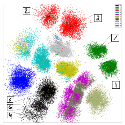
Application: Discovering Structure in Digits
Unsupervised learning can discover structure in digits without any labels.
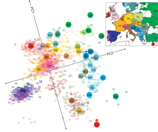
Application: DNA Analysis
Dimensionality reduction applied to DNA reveal the geography of European countries:
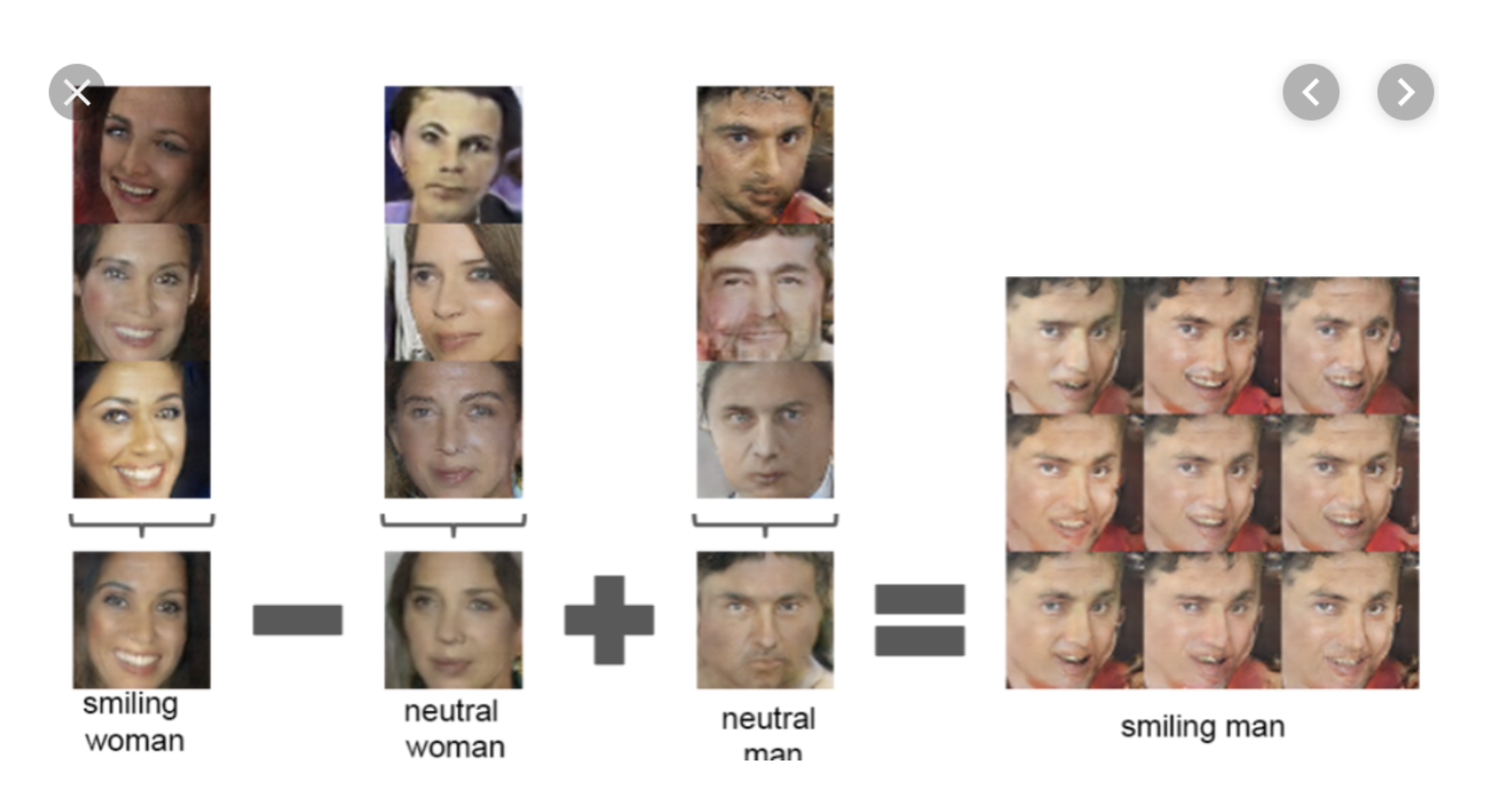
Application: Human Faces
Modern unsupervised algorithms based on deep learning uncover structure in human face datasets.
Unsupervised Learning in This Course
We will explore several types of unsupervised learning problems.
- Density estimation
- Anomaly and novelty detection
- Clustering
- Dimensionality Reduction
Next, we will start by setting up some notation.

Part 2: The Language of Unsupervised Learning
Next, let's look at how to define an unsupervised learning problem more formally.
Components of an Unsupervised Learning Problem
At a high level, an unsupervised machine learning problem has the following structure:
$$ \underbrace{\text{Dataset}}_\text{Attributes} + \underbrace{\text{Learning Algorithm}}_\text{Model Class + Objective + Optimizer } \to \text{Unsupervised Model} $$The unsupervised model describes interesting structure in the data. For instance, it can identify interesting hidden clusters.
Unsupervised Dataset: Notation
We define of size $n$ a dataset for unsupervised learning as $$\mathcal{D} = \{x^{(i)} \mid i = 1,2,...,n\}$$
Each $x^{(i)} \in \mathbb{R}^d$ denotes an input, a vector of $d$ attributes or features.
Data Distribution
We will assume that the dataset is sampled from a probability distribution $\mathbb{P}$, which we will call the data distribution. We will denote this as $$x \sim \mathbb{P}.$$
The dataset $\mathcal{D} = \{x^{(i)} \mid i = 1,2,...,n\}$ consists of independent and identicaly distributed (IID) samples from $\mathbb{P}$.
Data Distribution: IID Sampling
The key assumption in that the training examples are independent and identicaly distributed (IID).
- Each training example is from the same distribution.
- This distribution doesn't depend on previous training examples.
Example: Flipping a coin. Each flip has same probability of heads & tails and doesn't depend on previous flips.
Counter-Example: Yearly census data. The population in each year will be close to that of the previous year.
Components of an Unsupervised Learning Algorithm
We can think of a unsupervised learning algorithm as consisting of three components:
- A model class: the set of possible unsupervised models we consider.
- An objective function, which defines how good a model is.
- An optimizer, which finds the best predictive model in the model class according to the objective function
Model: Notation
We'll say that a model is a function $$ f : \mathcal{X} \to \mathcal{S} $$ that maps inputs $x \in \mathcal{X}$ to some notion of structure $s \in \mathcal{S}$.
Structure can have many definitions (clusters, low-dimensional representations, etc.), and we will see many examples.
Often, models have parameters $\theta \in \Theta$ living in a set $\Theta$. We will then write the model as $$ f_\theta : \mathcal{X} \to \mathcal{S} $$ to denote that it's parametrized by $\theta$.
Model Class: Notation
Formally, the model class is a set $$\mathcal{M} \subseteq \{f \mid f : \mathcal{X} \to \mathcal{S} \}$$ of possible models that map input features to structural elements.
When the models $f_\theta$ are paremetrized by parameters $\theta \in \Theta$ living in some set $\Theta$. Thus we can also write $$\mathcal{M} = \{f_\theta \mid f : \mathcal{X} \to \mathcal{S}; \; \theta \in \Theta \}.$$
Objective: Notation
To capture this intuition, we define an objective function (also called a loss function) $$J(f) : \mathcal{M} \to [0, \infty), $$ which describes the extent to which $f$ "fits" the data $\mathcal{D} = \{x^{(i)} \mid i = 1,2,...,n\}$.
When $f$ is parametrized by $\theta \in \Theta$, the objective becomes a function $J(\theta) : \Theta \to [0, \infty).$
Optimizer: Notation
An optimizer finds a model $f \in \mathcal{M}$ with the smallest value of the objective $J$. \begin{align*} \min_{f \in \mathcal{M}} J(f) \end{align*}
Intuitively, this is the function that bests "fits" the data on the training dataset.
When $f$ is parametrized by $\theta \in \Theta$, the optimizer minimizes a function $J(\theta)$ over all $\theta \in \Theta$.
An Example: $K$-Means
As an example, let's use the $K$-Means algorithm that we saw earlier.
Recall that:
- The algorithm seeks to find $K$ hidden clusters in the data.
- Each cluster is characterized by its centroid (its mean).
- The clusters reveal interesting structure in the data.
The $K$-Means Model
We can think of the model returned by $K$-Means as a function $$f_\theta : \mathcal{X} \to \mathcal{S}$$ that assigns each input $x$ to a cluster $s \in \mathcal{S} = \{1,2,\ldots,K\}$.
The parameters $\theta$ of the model are $K$ centroids $c_1, c_2, \ldots c_K \in \mathcal{X}$. The class of $x$ is $k$ if $c_k$ is the closest centroid to $x$.
The $K$-Means Objective
How do we determine whether $f_\theta$ is a good clustering of the dataset $\mathcal{D}$?
We seek centroids $c_k$ such that the distance between the points and their closest centroid is minimized: $$J(\theta) = \sum_{i=1}^n || x^{(i)} - \text{centroid}(f_\theta(x^{(i)})) ||,$$ where $\text{centroid}(k) = c_k$ denotes the centroid for cluster $k$.
The $K$-Means Optimizer
We can optimize this in a two stop process, starting with an initial random cluster assignment $f(x)$.
Repeat until convergence:
- Set each $c_k$ to be the center of the its cluster $\{x^{(i)} \mid f(x^{(i)}) = k\}$.
- Update clustering $f(x)$ such that $x^{(i)}$ is in the cluster of its closest centroid.
This is best illustrated visually (from Wikipedia):
Algorithm: K-Means
- Type: Unsupervised learning (clustering)
- Model family: $k$ centroids
- Objective function: Sum of distances to closest centroid
- Optimizer: Iterative optimization procedure.
Part 3: Unsupervised Learning in Practice
We will now look at some practical considerations to keep in mind when applying supervised learning.
Review: Data Distribution
We will assume that the dataset is sampled from a probability distribution $\mathbb{P}$, which we will call the data distribution. We will denote this as $$x \sim \mathbb{P}.$$
The dataset $\mathcal{D} = \{x^{(i)} \mid i = 1,2,...,n\}$ consists of independent and identicaly distributed (IID) samples from $\mathbb{P}$.
Review: Generalization
In machine learning, generalization is the property of predictive models to achieve good performance on new, heldout data that is distinct from the training set.
How does generalization apply to unsupervised learning?
Generalization in Unsupervised Learning
We can think of the data distribution as being the sum of two distinct components $\mathbb{P} = F + E$
- A signal component $F$ (hidden clusters, speech, low-dimensional data space, etc.)
- A random noise component $E$
A machine learning model generalizes if it fits the true signal $F$; it overfits if it learns the noise $E$.
An Unsupervised Learning Dataset
Consider the following dataset, consisting of a mixture of Gaussians.
import numpy as np
from sklearn import datasets
from matplotlib import pyplot as plt
plt.rcParams['figure.figsize'] = [12, 4]

np.random.seed(0)
X, y = datasets.make_blobs(centers=4)
plt.scatter(X[:,0], X[:,1])
<matplotlib.collections.PathCollection at 0x120073b38>

We know the true labels of these clusers, and we can visualize them.
plt.scatter(X[:,0], X[:,1], c=y)
<matplotlib.collections.PathCollection at 0x122d99b00>

Underfitting in Unsupervised Learning
Underfitting happens when we are not able to fully learn the signal hidden in the data.
In the context of $K$-Means, this means not capturing all the clusters in the data.
Let's run $K$-Means on our toy dataset.
# fit a K-Means
from sklearn import cluster
model = cluster.KMeans(n_clusters=2)
model.fit(X)
KMeans(n_clusters=2)
The centroids find two distinct components in the data, but they fail to capture the true structure.
plt.scatter(X[:,0], X[:,1], c=y)
plt.scatter(model.cluster_centers_[:,0], model.cluster_centers_[:,1], marker='D', c='r', s=100)
print('K-Means Objective: %.2f' % -model.score(X))
K-Means Objective: 462.03

Consider now what happens if we further increase the number of clusters.
Ks = [4, 10, 20]
f, axes = plt.subplots(1,3)
for k, ax in zip(Ks, axes):
    model = cluster.KMeans(n_clusters=k)
    model.fit(X)
    ax.scatter(X[:,0], X[:,1], c=y)
    ax.scatter(model.cluster_centers_[:,0], model.cluster_centers_[:,1], marker='D', c='r', s=100)
    ax.set_title('K-Means Objective: %.2f' % -model.score(X))

Overfitting in Unsupervised Learning
Overfitting happens when we fit the noise, but not the signal.
In our example, this means fitting small, local noise clusters rather than the true global clusters.
model = cluster.KMeans(n_clusters=50)
model.fit(X)
plt.scatter(X[:,0], X[:,1], c=y)
plt.scatter(model.cluster_centers_[:,0], model.cluster_centers_[:,1], marker='D', c='r', s=100)
print('K-Means Objective: %.2f' % -model.score(X))
K-Means Objective: 4.94

The Elbow Method
The Elbow method is a way of tuning hyper-parameters in unsupervised learning.
- We plot the objective function as a function of the hyper-parameter $K$.
- The "elbow" of the curve happens when its rate of decrease substantially slows down.
- The "elbow' is a good guess for the hyperparameter.
In our example, the decrease in objective values slows down after $K=4$, and after that the curve becomes just a line.
Ks, objs = range(1,11), []
for k in Ks:
    model = cluster.KMeans(n_clusters=k)
    model.fit(X)
    objs.append(-model.score(X))

plt.plot(Ks, objs, '.-', markersize=15)
plt.scatter([4], [objs[3]], s=200, c='r')
plt.xlabel("Number of clusters K")
plt.ylabel("Objective Function Value")
Text(0, 0.5, 'Objective Function Value')

Detecting Overfitting and Underfitting
In unsupervised learning, overfitting and underfitting are more difficult to quantify than in supervised learning.
- Performance may depend on our intuition and require human evaluation
- If we know the true labels, we can measure the accuracy of the clustering
If our model is probabilistic, we can detect overfitting without labels by comparing the log-likelihood between the training set and a holdout set (next lecture!).
Reducing Overfitting
There are multiple ways to control for overfitting:
- Reduce model complexity (e.g., reduce $K$ in $K$-Means)
- Penalize complexity in objective (e.g., penalize large $K$)
- Use a probabilistic model and regularize it.
Summary
The concept of generalization applies to both supervised and unsupervised learning.
- In supervised learning, it is easier to quantify via the accuracy.
- In unsupervised learning, we may not be able to easily detect overfitting, but it still happens.