Part 1: An Artifical Neuron
In this lecture, we will learn about a new class of machine learning algorithms inspired by the brain.
We will start by defining a few building blocks for these algorithms, and draw connections to neuroscience.
Review: Binary Classification
In supervised learning, we fit a model of the form $$ f : \mathcal{X} \to \mathcal{Y} $$ that maps inputs $x \in \mathcal{X}$ to targets $y \in \mathcal{Y}$.
In classification, the space of targets $\mathcal{Y}$ is discrete. Classification is binary if $\mathcal{Y} = \{0,1\}$
Review: Logistic Regression
Logistic regression fits a model of the form $$ f(x) = \sigma(\theta^\top x) = \frac{1}{1 + \exp(-\theta^\top x)}, $$ where $$ \sigma(z) = \frac{1}{1 + \exp(-z)} $$ is known as the sigmoid or logistic function.
A Biological Neuron
In order to define an artifical neuron, let's look first at a biological one.
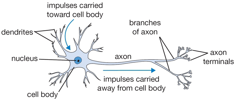
- Each neuron receives input signals from its dendrites
- If input signals are strong enough, neuron fires output along its axon, which connects to the dendrites of other neurons.
An Artificial Neuron: Example
We can imitate this machinery using an idealized artifical neuron.
- Dendrite $j$ gets signal $x_j$; modulates multiplicatively to $w_j \cdot x_j$.
- The body of the neuron sums the modulated inputs: $\sum_{j=1}^d w_j \cdot x_j$.
- These go into the activation function that produces an ouput.
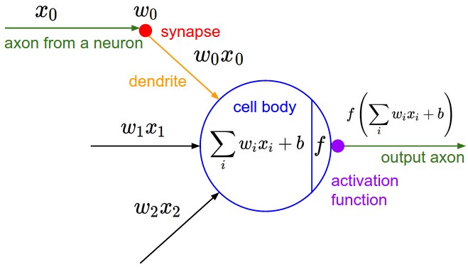
An Artificial Neuron: Notation
More formally, we say that a neuron is a model $f : \mathbb{R}^d \to [0,1]$, with the following components:
- Inputs $x_1,x_2,...,x_d$, denoted by a vector $x$.
- Weight vector $w \in \mathbb{R}^d$ that modulates input $x$ as $w^\top x$.
- An activation function $\sigma: \mathbb{R} \to \mathbb{R}$ that computes the output $\sigma(w^\top x)$ of the neuron based on the sum of modulated features $w^\top x$.
Perceptron
If we use a step function as the activation function, we obtain the classic Perceptron model:
$$ f(x) = \begin{cases} 1 & \text{if $\theta^\top x>0$}, \\ 0 & \text{otherwise} \end{cases} $$This models a neuron that fires if the inputs are sufficiently large, and doesn't otherwise.
We can visualize the activation function of the Perceptron.
step_fn = lambda z: 1 if z > 0 else 0
plt.plot(z, [step_fn(zi) for zi in z])
[<matplotlib.lines.Line2D at 0x120c11978>]

Logistic Regression as an Artifical Neuron
Logistic regression is a model of the form $$ f(x) = \sigma(\theta^\top x) = \frac{1}{1 + \exp(-\theta^\top x)}, $$ that can be interpreted as a neuron that uses the sigmoid as the activation function.
The sigmoid activation function encodes the idea of a neuron firing if the inputs exceed a threshold, makes make the activation function "smooth".
z = np.linspace(-5, 5)
sigma = 1/(1+np.exp(-z))

plt.plot(z, sigma)
[<matplotlib.lines.Line2D at 0x120c832e8>]

Activation Functions
There are many other activation functions that can be used. In practice, these two work better than the sigmoid:
- Hyperbolic tangent (
tanh): $\sigma(z) = \tanh(z)$ - Rectified linear unit (
ReLU): $\sigma(z) = \max(0, z)$
We can easily visualize these.
%matplotlib inline
import matplotlib.pyplot as plt
plt.rcParams['figure.figsize'] = [12, 4]

plt.subplot(121)
plt.plot(z, np.tanh(z))
plt.subplot(122)
plt.plot(z, np.maximum(z, 0))
[<matplotlib.lines.Line2D at 0x1333eb668>]

Classification Dataset: Iris Flowers
To demonstrate classification algorithms, we are going to use the Iris flower dataset.
We are going to define an artificial neuron for the binary classification problem (class-0 vs the rest).
# https://scikit-learn.org/stable/auto_examples/neighbors/plot_classification.html
import numpy as np
import pandas as pd
from sklearn import datasets

# Load the Iris dataset
iris = datasets.load_iris(as_frame=True)
iris_X, iris_y = iris.data, iris.target

# rename class two to class one
iris_y2 = iris_y.copy()
iris_y2[iris_y2==2] = 1

X = iris_X.to_numpy()[:,:2]
Y = iris_y2
This is a visualization of the dataset.
# Plot also the training points
p1 = plt.scatter(X[:,0], X[:,1], c=iris_y2, edgecolor='k', s=60, cmap=plt.cm.Paired)
plt.xlabel('Petal Length')
plt.ylabel('Petal Width')
plt.legend(handles=p1.legend_elements()[0], labels=['Setosa', 'Non-Setosa'], loc='lower right')
<matplotlib.legend.Legend at 0x12f4f45c0>

Below, we define neuron with a sigmoid activation function (and its gradient).
def neuron(X, theta):
    activation_fn = lambda z: 1/(1+np.exp(-z))
    return activation_fn(X.dot(theta))

def gradient(theta, X, y):
    return np.mean((y - neuron(X, theta)) * X.T, axis=1)
We can optimize is using gradient descent.
threshold = 5e-5
step_size = 1e-1

iter, theta, theta_prev = np.zeros((3,)), np.ones((3,)), 0
iris_X['one'] = 1 # add a vector of ones for the bias
X_train = iris_X.iloc[:,[0,1,-1]].to_numpy()
y_train = iris_y2.to_numpy()

while np.linalg.norm(theta - theta_prev) > threshold:
    if iter % 50000 == 0:
        print('Iteration %d.' % iter)
    theta_prev = theta
    grad = gradient(theta, X_train, y_train)
    theta = theta_prev + step_size * grad
    iter += 1
Iteration 0.
Iteration 50000.
Iteration 100000.
Iteration 150000.
Iteration 200000.
This neuron learns a linear decision boundary that separates the data.
# generate predictions over a grid:
xx, yy = np.meshgrid(np.arange(3.3, 8.9, 0.02), np.arange(1.0, 5.4, 0.02))
Z = neuron(np.c_[xx.ravel(), yy.ravel(), np.ones(xx.ravel().shape)], theta)
Z[Z<0.5] = 0
Z[Z>=0.5] = 1

# Put the result into a color plot
Z = Z.reshape(xx.shape)
plt.pcolormesh(xx, yy, Z, cmap=plt.cm.Paired)

# Plot also the training points
plt.scatter(X[:, 0], X[:, 1], c=Y, edgecolors='k', cmap=plt.cm.Paired)
plt.xlabel('Sepal length')
plt.ylabel('Sepal width')
Text(0, 0.5, 'Sepal width')

Algorithm: Artificial Neuron
- Type: Supervised learning (regression and classification).
- Model family: Linear model followed by non-linear activation.
- Objective function: Any differentiable objective.
- Optimizer: Gradient descent.
- Special Cases: Logistic regression, Perceptron

Part 2: Artificial Neural Networks
Let's now see how we can connect neurons into networks that form complex models that further mimic the brain.
Review: Artificial Neuron
We say that a neuron is a model $f : \mathbb{R}^d \to [0,1]$, with the following components:
- Inputs $x_1,x_2,...,x_d$, denoted by a vector $x$.
- Weight vector $w \in \mathbb{R}^d$ that modulates input $x$ as $w^\top x$.
- An activation function $\sigma: \mathbb{R} \to \mathbb{R}$ that computes the output $\sigma(w^\top x)$ of the neuron based on the sum of modulated features $w^\top x$.
Review: Logistic Regression as Neuron
Logistic regression is a model of the form $$ f(x) = \sigma(\theta^\top x) = \frac{1}{1 + \exp(-\theta^\top x)}, $$ that can be interpreted as a neuron that uses the sigmoid as the activation function.
Neural Networks: Intuition
A neural network is a directed graph in which a node is a neuron that takes as input the outputs of the neurons that are connected to it.
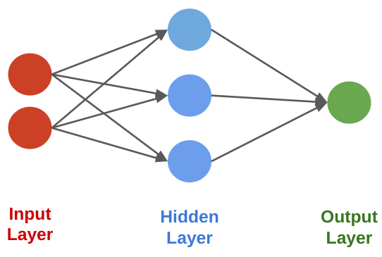
Neural Networks: Layers
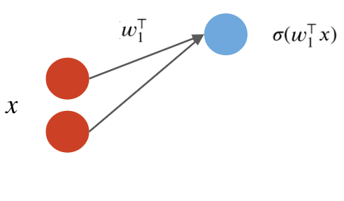
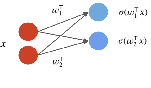
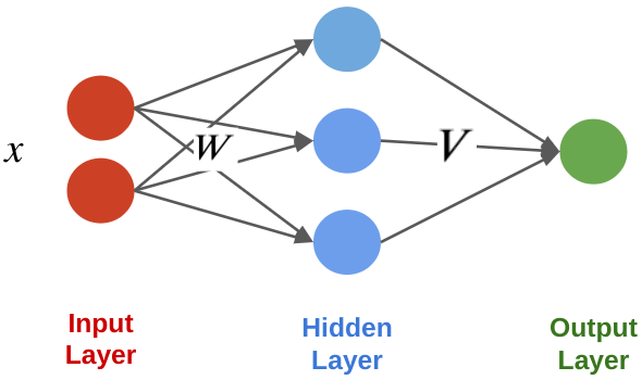
A neural network layer is a model $f : \mathbb{R}^d \to \mathbb{R}^p$ that applies $p$ neurons in parallel to an input $x$. $$ f(x) = \begin{bmatrix} \sigma(w_1^\top x) \\ \sigma(w_2^\top x) \\ \vdots \\ \sigma(w_p^\top x) \end{bmatrix}. $$ where each $w_k$ is the vector of weights for the $k$-th neuron. We refer to $p$ as the size of the layer.
The first output of the layer is a neuron with weights $w_1$:
The second neuron has weights $w_2$:
The third neuron has weights $w_3$:
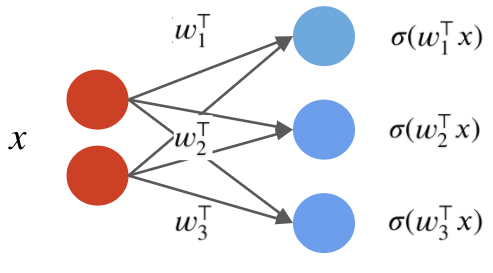
The parameters of the layer are $w_1, w_2, w_3$.
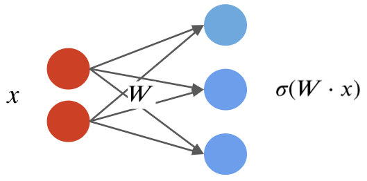
By combining the $w_k$ into one matrix $W$, we can write in a more succinct vectorized form: $$f(x) = \sigma(W\cdot x) = \begin{bmatrix} \sigma(w_1^\top x) \\ \sigma(w_2^\top x) \\ \vdots \\ \sigma(w_p^\top x) \end{bmatrix}, $$ where $\sigma(W\cdot x)_k = \sigma(w_k^\top x)$ and $W_{kj} = (w_k)_j$.
Visually, we can represent this as follows:
Neural Networks: Notation
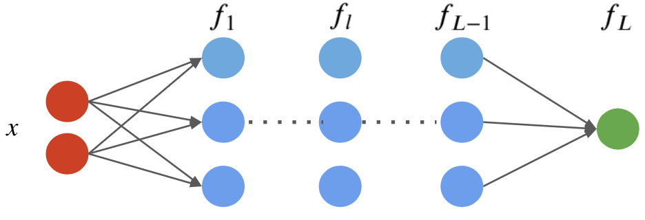
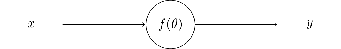
A neural network is a model $f : \mathbb{R}^d \to \mathbb{R}$ that consists of a composition of $L$ neural network layers: $$ f(x) = f_L \circ f_{L-1} \circ \ldots f_l \circ \ldots f_1 (x). $$ The final layer $f_L$ has size one (assuming the neural net has one ouput); intermediary layers $f_l$ can have any number of neurons.
The notation $f \circ g(x)$ denotes the composition $f(g(x))$ of functions.
We can visualize this graphically as follows.
This implementation looks as follows.
# a two layer network with logistic function as activation
class Net():
    def __init__(self, x_dim, W_dim):
        # weight matrix for layer 1
        self.W = np.random.normal(size=(x_dim, W_dim))
        # weight matrix for layer 2, also the output layer
        self.V = np.random.normal(size=(W_dim, 1))
        # activation function
        self.afunc = lambda x: 1/(1+np.exp(-x))

    def predict(self, x):
        # get output of the first layer
        l1 = self.afunc(np.matmul(x, self.W))
        # get output of the second layer, also the output layer
        out = self.afunc(np.matmul(l1, self.V))
        return out
Later in this lecture, we will see how to train this model using gradient descent.
Types of Neural Network Layers
There are many types of neural network layers that can exist. Here are a few:
- Ouput layer: normally has one neuron and special activation function that depends on the problem
- Input layer: normally, this is just the input vector $x$.
- Hidden layer: Any layer between input and output.
- Dense layer: A layer in which every input is connected to every neuron.
- Convolutional layer: A layer in which the operation $w^\top x$ implements a mathematical convolution.
- Recurrent Layer: A layer in which a neuron's output is connected back to the input.
Algorithm: (Fully-Connected) Neural Network
- Type: Supervised learning (regression and classification).
- Model family: Compositions of layers of artificial neurons.
- Objective function: Any differentiable objective.
- Optimizer: Gradient descent.
Pros and Cons of Neural Nets
Neural networks are very powerful models.
- They are flexible, and can approximate any function.
- They work well over unstructured inputs like audio or images.
- They can achieve state-of-the-art perfomrance.
They also have important drawbacks.
- They can also be slow and hard to train.
- Large neworks require a lot of data.
Part 3: Backpropagation
We have defined what is an artificial neural network.
Let's now see how we can train it so that it performs well on given tasks.
Review: Neural Network Layers
A neural network layer is a model $f : \mathbb{R}^d \to \mathbb{R}^p$ that applies $p$ neurons in parallel to an input $x$. $$f(x) = \sigma(W\cdot x) = \begin{bmatrix} \sigma(w_1^\top x) \\ \sigma(w_2^\top x) \\ \vdots \\ \sigma(w_p^\top x) \end{bmatrix}, $$ where each $w_k$ is the vector of weights for the $k$-th neuron and $W_{kj} = (w_k)_j$. We refer to $p$ as the size of the layer.
Review: Neural Networks
A neural network is a model $f : \mathbb{R} \to \mathbb{R}$ that consists of a composition of $L$ neural network layers: $$ f(x) = f_L \circ f_{L-1} \circ \ldots f_1 (x). $$ The final layer $f_L$ has size one (assuming the neural net has one ouput); intermediary layers $f_l$ can have any number of neurons.
The notation $f \circ g(x)$ denotes the composition $f(g(x))$ of functions
We can visualize this graphically as follows.
Review: The Gradient
The gradient $\nabla_\theta f$ further extends the derivative to multivariate functions $f : \mathbb{R}^d \to \mathbb{R}$, and is defined at a point $\theta$ as $$ \nabla_\theta f (\theta) = \begin{bmatrix} \frac{\partial f(\theta)}{\partial \theta_1} \\ \frac{\partial f(\theta)}{\partial \theta_2} \\ \vdots \\ \frac{\partial f(\theta)}{\partial \theta_d} \end{bmatrix}.$$ In other words, the $j$-th entry of the vector $\nabla_\theta f (\theta)$ is the partial derivative $\frac{\partial f(\theta)}{\partial \theta_j}$ of $f$ with respect to the $j$-th component of $\theta$.
Review: Gradient Descent
If we want to optimize an objective $J(\theta)$, we start with an initial guess $\theta_0$ for the parameters and repeat the following update until the function is no longer decreasing: $$ \theta_i := \theta_{i-1} - \alpha \cdot \nabla_\theta J(\theta_{i-1}). $$
As code, this method may look as follows:
theta, theta_prev = random_initialization()
while norm(theta - theta_prev) > convergence_threshold:
    theta_prev = theta
    theta = theta_prev - step_size * gradient(theta_prev)
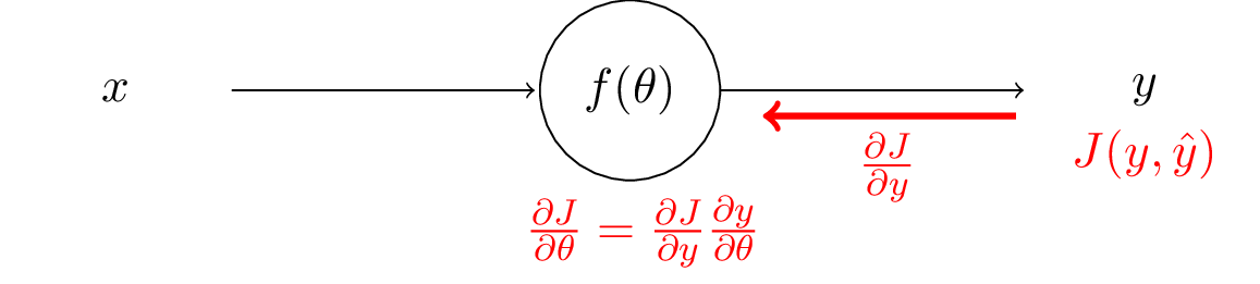
Backpropagation
To apply gradient descent, we need to calculate gradients for every parameter in a neural network model $f$: $$\frac{\partial J}{\partial \theta_0}, \frac{\partial J}{\partial \theta_1}, \cdots, \frac{\partial J}{\partial \theta_d}$$
It might be possible to do it manually when the network is small. But it is nearly impossible and very much error-prone to compute gradients for larger networks.
Backpropagation is a way of calculating gradients efficiently for neural network models with arbitrary number of layers and neurons.
The core idea of it is something we are actually very familiar with: the chain rule.
Review: Chain Rule of Calculus
If we have two differentiable functions $f(x)$ and $g(x)$, and $$F(x) = f \circ g (x)$$ then the derivative of $F(x)$ is: $$ F^\prime (x) = f^\prime (g(x)) \cdot g^\prime (x).$$
Let $y=f(u)$ and $u=g(x)$, we also have: $$ \frac{dy}{dx} = \frac{dy}{du} \frac{du}{dx}.$$
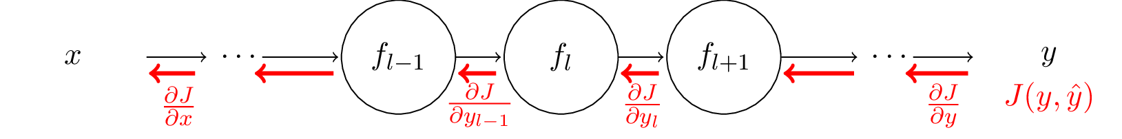
Chain Rule in Neural Nets
A neural network is a model $f : \mathbb{R} \to \mathbb{R}$ that consists of a composition of $L$ neural network layers: $$ f(x) = f_L \circ f_{L-1} \circ \ldots f_1 (x). $$
Let $y_l$ denote the output $f_l \circ f_{-1} \circ f_1(x)$ of layer $l$.
The chain rule tells us to compute $\frac{\partial J}{\partial \theta_l}$ for all parameters $\theta_l$ in layer $l$. We can break the computation down as: $$ \frac{\partial J}{\partial \theta_l} = \frac{\partial J}{\partial y_L} \frac{\partial y_L}{\partial y_{L-1}} \cdots \frac{\partial y_{l+1}}{\partial y_l} \frac{\partial y_l}{\partial \theta_l}, $$ where $y_L, y_{L-1} \cdots y_l$ are the outputs from each layer.
Note that the computation of $\frac{\partial J}{\partial y_l}$ can be re-used for computing gradients for all $\theta$ in layers before $l$.
This is the key idea of backpropagation: local gradients computation for each layer can be 'chained' to obtain gradients.
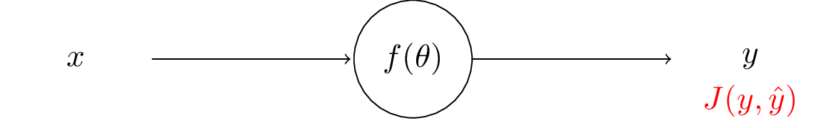
With the output $y$, target label $\hat{y}$, and loss function $J$, we can compute the loss (error) of the prediction.
The backpropagation starts from the output layer and moves backwards.
We first need to compute the gradients of the loss to the output.
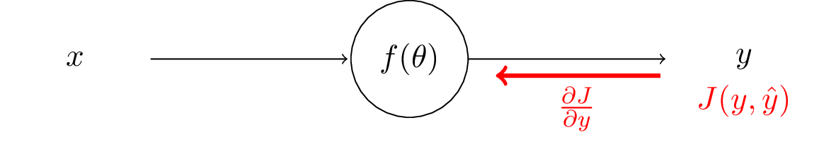
After we have those, then using the chain rule, we can compute the gradients with respect to the network parameters $\theta$.
We can keep working upstream and compute gradients to the input. After that we finish the backpropagation in this layer.
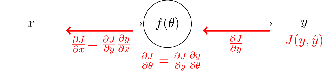
We can apply this process recursively to obtain derivatives for any number of layers.
Backprogragation by Hand
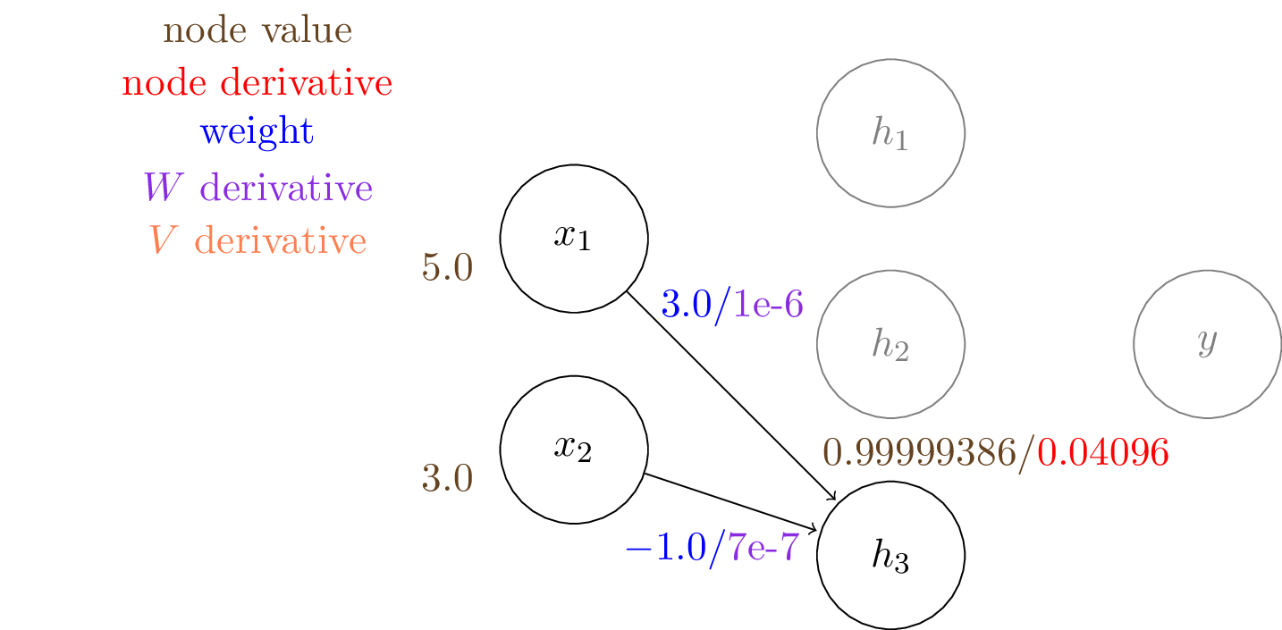
Let's work out by hand what backpropagation would do on our two layer neural network.
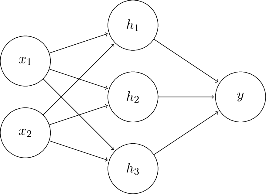
For our two layer fully connected network with sigmoid activation, the network is composed of following functions:
$$\mathbf{h} = \sigma(\mathbf{W}^T \mathbf{x})$$$$y = \sigma(\mathbf{V}^T \mathbf{h}),$$where $\mathbf{x} = [x_1,x_2]^T, \mathbf{h} = [h_1,h_2,h_3]^T, \mathbf{W} \in \mathbb{R}^{2\times3}, \mathbf{V} \in \mathbb{R}^{3\times1}$, and $\sigma$ is the sigmoid function.
In our example, we have the following values:
$\mathbf{x} = [5.0,3.0]^T,~~~~\hat{y} = 1$ means it is positive class.
$\mathbf{W} = \begin{bmatrix} 1.0 & -1.0 & 3.0\\ 2.0 & 2.0 & -1.0 \end{bmatrix}$
$\mathbf{V} = [0.1,0.5,-0.1]^T$
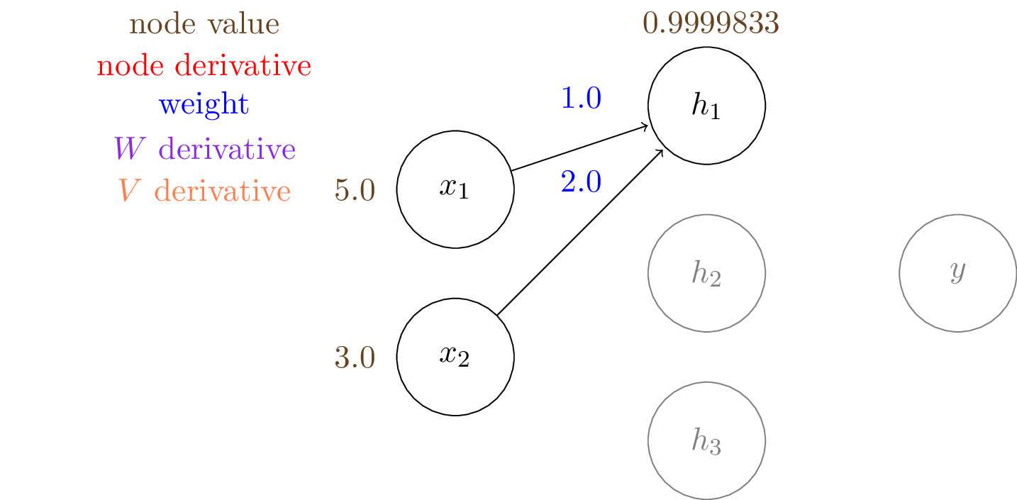
$h_1 = \sigma (W_{11} \cdot x_1 + W_{21} \cdot x_2) = \sigma (1.0\times5.0 + 2.0\times3.0) = 0.99998329857$
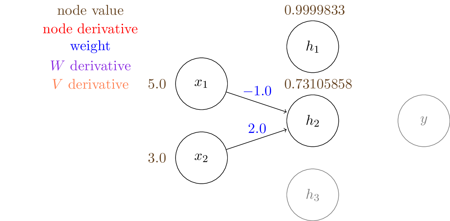
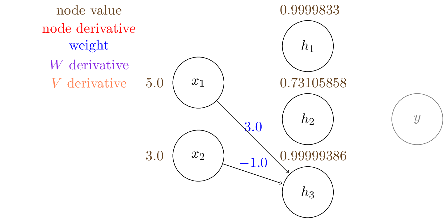
We can compute the output of the hidden layer, $\mathbf{h}$: \begin{align*} h_1 &= \sigma (W_{11} \cdot x_1 + W_{21} \cdot x_2) = \sigma (1.0\times5.0 + 2.0\times3.0) = 0.9999 \\ h_2 &= \sigma (W_{12} \cdot x_1 + W_{22} \cdot x_2) = \sigma (-1.0\times5.0 + 2.0\times3.0) = 0.7310 \\ h_3 &= \sigma (W_{13} \cdot x_1 + W_{23} \cdot x_2) = \sigma (3.0\times5.0 + -1.0\times3.0) = 0.9999 \end{align*}
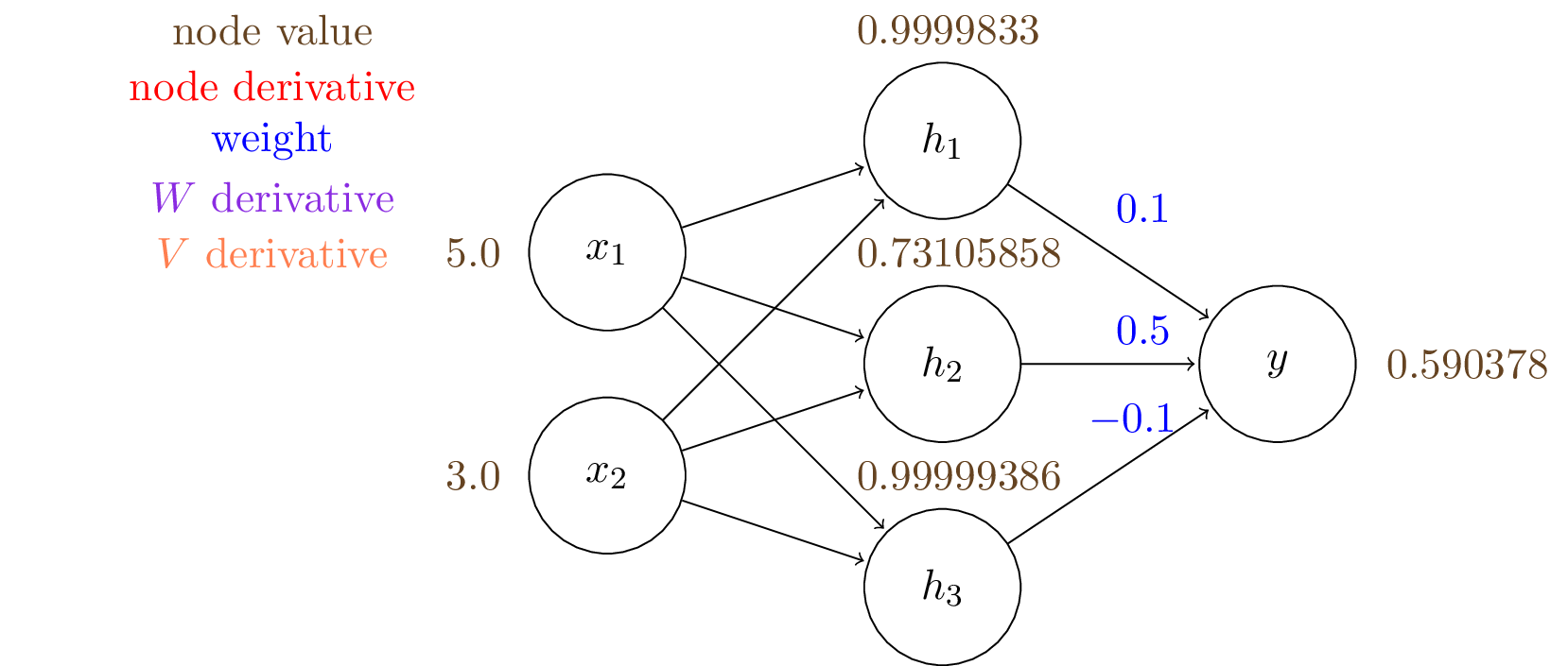
$y = \sigma (V_1 \cdot h_1 + V_2 \cdot h_2 + V_3 \cdot h_3) = 0.590378$
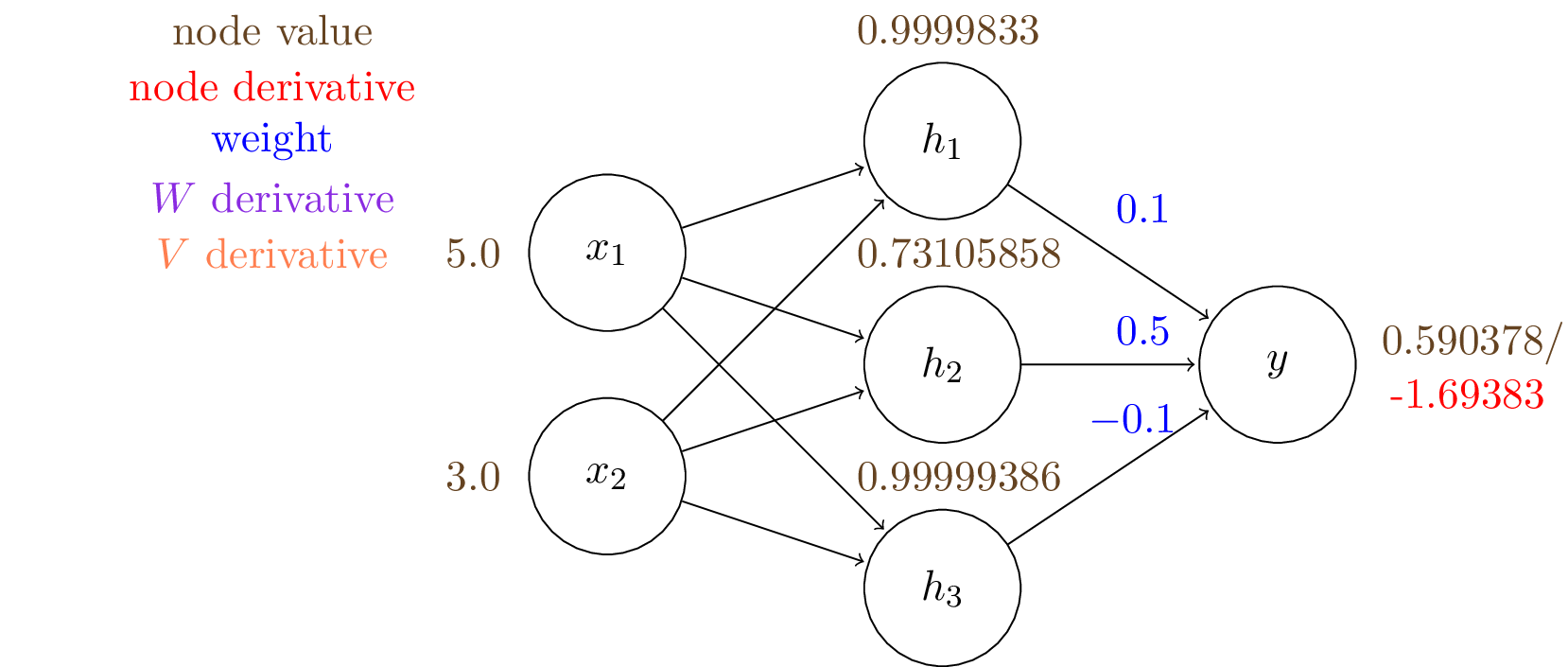
We can also compute the gradient (shown in red): $\frac{\mathrm{d}J}{\mathrm{d}{y}} = - 1/y = -1.69383$
We are now ready to kick start the backpropagation steps.
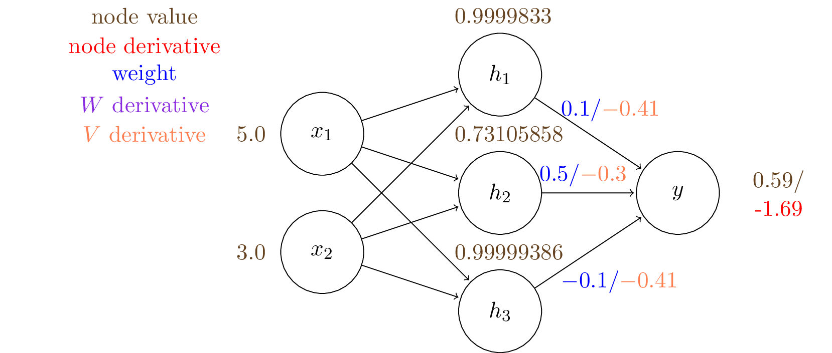
Next, we want to compute gradients at the hidden layer:
$$\frac{\mathrm{d}J}{\mathrm{d}{h}} = \frac{\mathrm{d}J}{\mathrm{d}{y}} \frac{\mathrm{d}y}{\mathrm{d}{h}}$$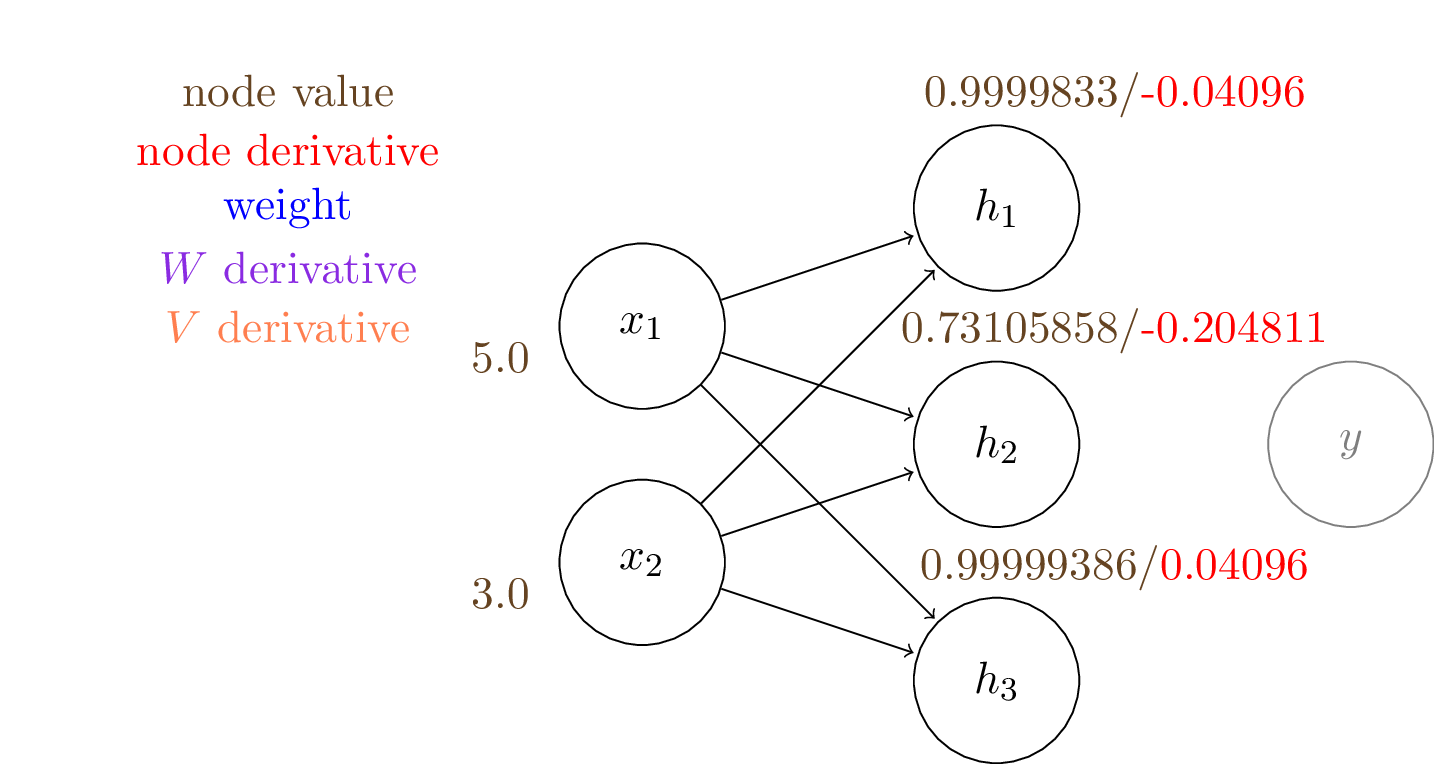
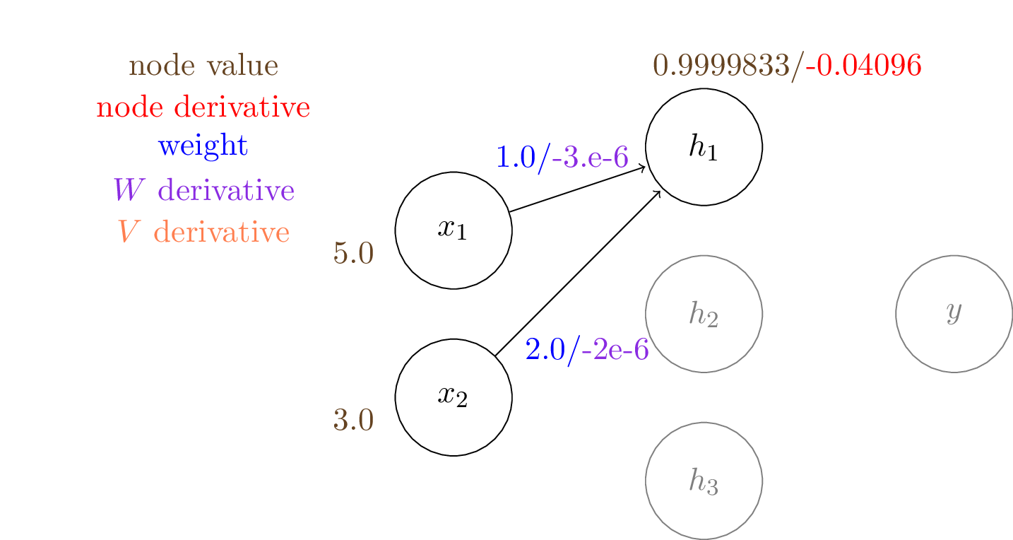
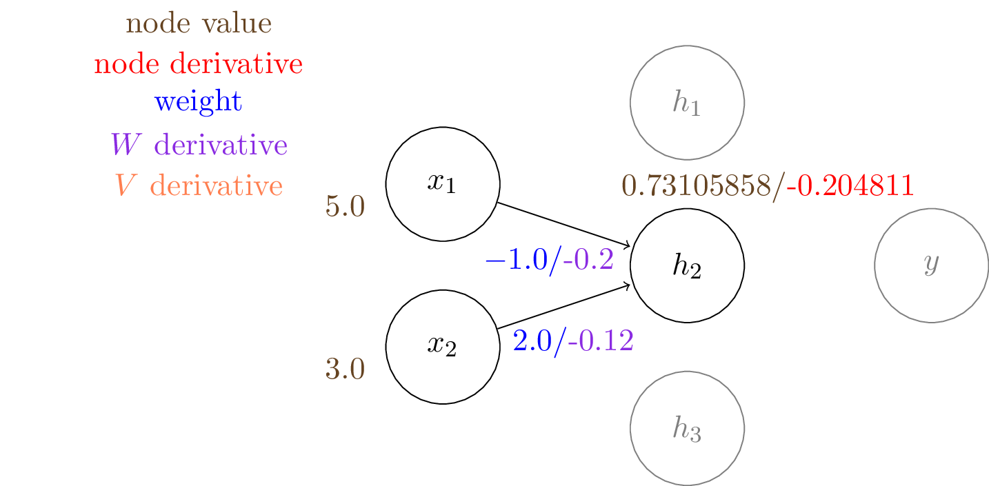
Note the gradients to the weights connecting to $h_2$ are larger in magnitude than others.
And now we have the gradients to all the learnable weights in this two layer network and we can tune the weights by gradient descenet.
The gradients tell us how much to change for each weight so that the loss will become smaller.
Now let's implement backprop with the simple neural network model we defined earlier.
We start by implementing the building block of our network: a linear layer with sigmoid activation.
import numpy as np

# a single linear layer with sigmoid activation
class LinearSigmoidLayer():
    def __init__(self, in_dim, out_dim):
        self.W = np.random.normal(size=(in_dim,out_dim))
        self.W_grad = np.zeros_like(self.W)

        self.afunc = lambda x: 1. / (1. + np.exp(-x))

    # forward function to get output
    def forward(self, x):
        Wx = np.matmul(x, self.W)
        self.y = self.afunc(Wx)
        self.x = x
        return self.y

    # backward function to compute gradients
    def backward(self, grad_out):
        self.W_grad = np.matmul(
            self.x.transpose(),
            self.y * (1-self.y) * grad_out,
            )
        grad_in = np.matmul(
            self.y * (1-self.y) * grad_out,
            self.W.transpose()
            )

        return grad_in
Then we can stack the single layers to construct a two layer network.
# a two layer network with logistic function as activation
class Net():
    def __init__(self, x_dim, W_dim):
        self.l1 = LinearSigmoidLayer(x_dim, W_dim)
        self.l2 = LinearSigmoidLayer(W_dim, 1)

    # get output
    def predict(self, x):
        h = self.l1.forward(x)
        self.y = self.l2.forward(h)
        return self.y

    # backprop
    def backward(self, label):
        # binary cross entropy loss, and gradients
        if label == 1:
            J = -1*np.log(self.y)
            dJ = -1/self.y
        else:
            J = -1*np.log(1-self.y)
            dJ = 1/(1-self.y)

        # back propagation
        dJdh = self.l2.backward(dJ) # output --> hidden
        dJdx = self.l1.backward(dJdh) # hidden --> input
        return J

    # update weights according to gradients
    def grad_step(self, lr=1e-4):
        self.l1.W -= lr*self.l1.W_grad
        self.l2.W -= lr*self.l2.W_grad
We can run with our previous example to check if the results are consistent with our manual computation.
model = Net(2, 3)
model.l1.W = np.array([[1.0,-1.0,3.0],[2.0,2.0,-1.0]])
model.l2.W = np.array([[0.1],[0.5],[-0.1]])

x = np.array([5.0, 3.0])[np.newaxis,...]
x_label = 1

# forward
out = model.predict(x)

# backward
loss = model.backward(label=x_label)

print('loss: {}'.format(loss))
print('W grad: {}'.format(model.l1.W_grad))
print('V grad: {}'.format(model.l2.W_grad))
loss: [[0.52699227]]
W grad: [[-3.42057777e-06 -2.01341432e-01  1.25838681e-06]
 [-2.05234666e-06 -1.20804859e-01  7.55032084e-07]]
V grad: [[-0.40961516]
 [-0.29945768]
 [-0.40961948]]
Another sanity check is to perform gradient descent on the single sample input and see if we can achieve close to zero loss.
You can try to change the target label below to see the network is able to adapt in either case.
## gradient descent
loss = []
score = []
for i in range(100):
    out = model.predict(x)
    loss.append(model.backward(label=1)) # 1 for positive, 0 for negative
    model.grad_step(lr=1e-1)
    score.append(out)

import matplotlib.pyplot as plt
plt.plot(np.array(loss).squeeze(),'-')
plt.plot(np.array(score).squeeze(),'.')
[<matplotlib.lines.Line2D at 0x7f8c0ed09f10>]

Summary
- Neural networks are powerful models that can approximate any function.
- They are trained using gradient descent.
- In order to compute gradients, we use an efficient algorithm called backpropagation.